VOQC: Value Oriented Quality Control in Seismic Processing

We illustrate the importance of value orientation during the quality control efforts taken while performing seismic processing, and name our approach VOQC, or value oriented quality control. Quality control tests are run frequently during seismic processing. Our VOQC approach does not eliminate or act as substitution for current quality control methods, but could be characterized as attention to the value or the usefulness of any of the individual processing steps or of the processing as a whole. The value of the processes and processing as a whole has largely been implied in the past: if a process is superior at whatever it is supposed to do, then it must be more valuable. With the implied value taken for granted, we have therefore typically focussed our attention on the specific process being studied. It is the suggestion of this work that it is advisable to make the implicit value more explicit by paying specific attention to the value that our processes may give rise to. The VOQC concept also complements the decision analysis notion that the value of imperfect information such as seismic is related to the reliability of that information.

We make reference to some of the examples of VOQC in the literature, and show the VOQC method in a case study of unbiased surface consistent scaling. This leads us to describe some of the ways in which VOQC should be done in the current state of business and technology. Our key suggestions are:

1. Quality control maps should be made on economically relevant targets rather than exclusively upon windows that are large and whose economic relevance is indefinable.
2. Control experiments should be occasionally run on crucial processes such that the effect of the crucial process can be measured on the final processing output and upon an economically relevant target.
3. Continuous evaluation of the amplitude characteristics of the data should be performed, focussed on an economically relevant target, throughout the processing sequence. In the case of data with an AVO or azimuthal amplitude/travel time (azimuthal) goal, the AVO or azimuthal characteristics of the data should be studied in this manner.

Processing and the Primacy of Value

The uses and goals of exploration seismic have changed. Seismic was originally used for structure alone. Eventually, and with increasing sophistication over time, the use of seismic data was extended to consider the reservoir. At present, seismic is used for AVO studies to a large degree; so much so that AVO and azimuthal studies are on the cusp of becoming standard end goals of the seismic program. Given that our goals, uses and objectives, for seismic have changed, should we not recognize this in our approach to processing the data? If our end product is an AVO inversion, should we not be thinking about, and evaluating, our progress relative to that eventual use from the beginning of the processing sequence to the end?

In consideration of this Value Special Edition, let us modify our language: the end use orientation we propose is in fact a value orientation. It follows that the value of a particular process is contained in its incremental contribution to the value of the final processed product and the use of that final product. The VOQC addition to quality control in processing is an extra element of value orientation, and as such will often require the participation of the interpreter or end user of the data. The VOQC approach thus calls for two things:

• That we keep the end, or value, in mind at all times when we process seismic data.
• That our processing should be an integrated effort between processor and interpreter.

To some degree, VOQC thinking has already begun to take root in seismic processing. AVO oriented quality control is starting to be used more commonly at a variety of commercial processing companies. This is heartening. It is hoped that this paper can help encourage this evolution. As a challenge to industry, let us not see a new noise attenuation, phase, pre-stack scaling or resolution process be discussed in the literature or marketed to industry without careful study and demonstration of its effect on a potential target or on the potential end use of the data.

VOQC in the Literature

Explicit value oriented processing has been illustrated to some degree in the literature. Schmidt et al. (2013) showed the importance of preconditioning the processed data to produce superior AVO results. While that work did not explicitly illustrate value, it did focus on the end use of the data, which was an elastic study. We would also suggest that work such as in Schmidt et al. (2013) should be done during the regular processing of the data rather than after the fact. These suggestions aside, Schmidt et al. (2013) was oriented to value and is a good example of some of the thinking that should be done. Similarly, work on end use quality control tools such as Common-Offset-Common-Azimuth (COCA) and Common-Azimuth-Common-Offset (CACO) displays for azimuthal studies also have value orientation.

Araman et al (2012) and Araman and Paternoster (2014) offer an excellent and well thought out perspective on VOQC. Their work is entirely focussed on the attributes that will be produced from the data and how to ensure that the data quality is as apt as possible for those attributes. The thinking of Araman and Paternoster (2014) is attribute oriented, rather than directly value oriented, and comes with its own set of acronyms. The orientation and language notwithstanding, their work amounts to a philosophy not dissimilar in many respects to the one we present in this paper. It is worth noting that Araman and Paternoster (2014) focus on heavily on AVO and AVAz consistency quality control in their work.

Hunt et al. (2008, 2010, 2012) outlined a complete VOQC argument for the Viking in West Central Alberta. In this work, a control experiment was conducted to determine the effect of 5D interpolation on the fidelity of pre-stack imaged gathers for AVO analysis of the Viking reservoir. Control was achieved by reprocessing the data numerous times with and without interpolation or other similar processes. Each data volume was otherwise treated identically and underwent identical AVO analysis procedures, and interpreted with identical objective methods. The work was evaluated at key wells by comparison of real data to synthetic gathers, and was evaluated on 2D line extractions tying those wells. The work was also evaluated by comparing AVO maps, and by objectively comparing the AVO map data to Viking porosity thickness data (phi-h) in the wells of the study area. The key thing that this work showed was the difference in the predictive capability of the end product with and without interpolation. Since the end product was the AVO prediction of an economic target, this exercise spoke to real value. Numerous wells were drilled with the interpolation-AVO approach, and the results of this new approach were evaluated in Hunt et al. (2012). In this work, scatterplots of the seismic predictions versus the Viking phi-h were compared. These scatterplots showed, in a fashion similar to that illustrated in all of the Viking papers noted here, that the interpolation-AVO approach had a higher correlation to phi-h and less scatter. The interpolation-AVO approach was shown to be more accurate. The value of this greater accuracy was estimated through evaluation of the modeled well performance itself. Table 1 summarizes that evaluation.

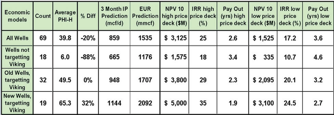
In the evaluation, an independent expert (Scott Hadley, VP Exploration of Fairborne Energy) determined whether wells were drilled targeting Viking or not, and further, whether seismic was used in the picking of the wells, and lastly whether the seismic method would have been the old stack amplitude method described in the literature or the new interpolation-AVO method. The interpolation-AVO method had, by a wide margin, the highest net present value (NPV). The difference was greater than a million dollars per well. The economics were run using the price deck of the time, which is much higher than today’s, and thus the results suggest a higher value difference than we would see today. The results directly estimate the value of the interpolation-AVO approach relative to the other approaches. These results also indirectly suggest a value to the greater accuracy of the gathers and the scatterplots. This evidence has led to a motto given in the recent Value of Integrated Geophysics (VIG) Doodletrain course, which is:

Accuracy = $

We argue that the notion of accuracy in seismic processing may have a general relationship to economic value based upon decision analysis. In Hunt (2013), decision analysis is used to show that economic value may be very sensitive to the reliability of imperfect information such as seismic data. The level of this sensitivity is also controlled by the relevance of the information to the economic outcome. It is for this reason that Hunt (2014), in part 1 of the Doodletrain VIG course, states that the value of seismic is inherently tied up in the reliability and relevance of the data. VOQC methods tie processing to value oriented outcomes and therefore seek to track the relevance and reliability of the processing, and hence the value of the work.

The complete assessment of value of processing that was illustrated in the Hunt et al. (2012) paper is rare in the literature due to the difficulty involved in carrying out complete control tests, as well as the challenges in modeling the economic impact of any particular process. Nevertheless, Downton et al. (2012) performed a similar control experiment for interpolation and Azimuthal AVO. To a certain degree, the accuracy-economic demonstration for AVO of Hunt et al. (2012) can be used as potential (analogous) economic evidence to support any process that improves AVO accuracy.

A VOQC Case Study Example for Unbiased Scaling

This case study example is an excerpt from a paper given at the 2014 CSEG Symposium. That presentation explored the uses and findings of a VOQC analysis of Cary and Nagarajappa’s (2013a, b) unbiased surface consistent scaling method. Cary and Nagarajappa (2013a, b) suggest that an improved scaling should yield superior amplitudes on horizons and AVO results. Our VOQC analysis of their new process targets the Viking sandstone and takes place on a subset of the data from Hunt et al. (2008, 2010, and 2012). This particular target and data are used since the effect of AVO accuracy has been demonstrated for it already, as described earlier in this article. The subset of the data is 116 square kilometers in size and contains 40 wells, many with full waveform sonic logs. Our VOQC evaluation has two parts:

1. A multi-well map evaluation, using all deep control, of the unbiased scaling method and its effect on AVO analysis.
2. An end-use oriented evaluation of the AVO response throughout the processing sequence using one key producing well with a full wire line log suite including a dipole log.

VOQC and Maps

The results of Cary and Nagarajappa’s (2013a, b) unbiased surface consistent scaling method were presented in the map domain, but without reference to target or value. In Figure 1 we show both the processor quality control similar to that in Cary and Nagarajappa’s (2013 a, b), as well as a VOQC set of maps. In Figure 1(a), we have an average absolute value amplitude map that uses data from 1.0 to 2.1 seconds. This is typical processor quality control, and is actually what the processor first delivered to the client on this project. The map is on the old, or biased, surface consistent scaling of the data, and shows strong amplitudes in red. This kind of map would be compared to the unbiased scaling equivalent as a kind of control experiment. The large 1.0 to 2.1 second window is typical of processor quality control techniques: its big window evaluates the general data trends quite well. This kind of processor quality control is very necessary, however it lacks any connection to the geology, to economic impact, to the specific goals of the project, and to an objective method of validation. Figure 1(b) is the biased amplitude map on the Wabamun peak, as picked by the interpreter. The Wabamun level geology is expected to be relatively invariant in the area, so a relatively invariant amplitude map was expected. The Wabamun peak shows similar amplitude patterns as in the processor quality control. A yellow arrow points out an area of high amplitudes in the lower left corner of the map area. Figure 1(c) is the unbiased amplitude map on the Wabamun peak. The high amplitude area in the lower left corner of the map is now absent. This change in map amplitude is thought to support a long wavelength improvement in the amplitudes due to the unbiased methodology. This horizon specific quality control is a step in the value direction since it appeals to geologic expectation, but still lacks value specificity. In Hunt et al. (2008, 2010) it was shown that good Viking reservoir will typically be expressed on the stack by lower amplitudes. Figure 1(d) is the stacked amplitude map at the Viking as processed with the old biased scaling. This map also shows some of the amplitude effects as on the processor quality control and on the Wabamun amplitude map, such as the high amplitude region in the lower left corner of the map area. Figure 1(e) is the stacked amplitude map at the Viking as processed with the new unbiased scaling. This map shows differences in amplitude patterns to that of the three other amplitude maps. The high amplitude area is absent. It can be argued qualitatively that in Figure 1(e) the low amplitude pattern associated with the Viking reservoir is more evenly discriminated from the non-reservoir above and below the producing area. Figures 1(d) and 1(e) represent the VOQC map method because they carry the evaluation of unbiased scaling to the economic target.

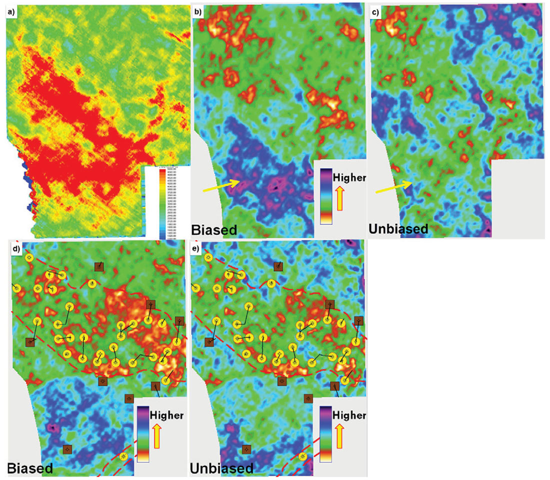
There is another important difference in the map images of Figure 1: the wells with an indication of reservoir quality were only shown in Figure 1(d) and 1(e). Integrating knowledge of the target reservoir to the amplitude map is an obvious but important thing to do in evaluating the effect of a process. There are 40 wells on this subset of the 3D survey, and each well has a phi-h measure assigned to it from the geosciences team. The producing fairway is defined loosely by the red dashed lines. In the 2014 CSEG Symposium presentation, we showed a variety of AVO maps with and without biased scaling. Those maps showed similar amplitude effects to those seen in Figure 1(d) and 1(e), but for brevity are not shown here. These qualitative map comparisons are encouraging, but how can we quantitatively demonstrate that one method yields more accurate amplitudes than another?

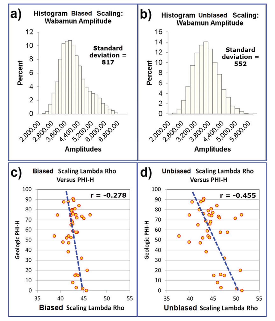
Figure 2 illustrates two different attempts to objectively determine the most reliable and most valuable processing methodology. Figure 2(a) shows the histogram of the Wabamun amplitudes for the biased scaling method over the entire mapped area. Figure 2(b) shows the histogram of the Wabamun amplitudes for the unbiased scaling method. These histograms make two things apparent: firstly that the unbiased method yields amplitudes with a smaller standard deviation for the Wabamun, and secondly that the unbiased scaling method also has less skew and has a more Gaussian appearance. If our assumption that the Wabamun amplitudes should be relatively invariant is correct, then the smaller standard deviation would seem to suggest that the unbiased scaling method is more accurate. We do not know whether the histogram should be Gaussian in appearance or not. This evidence is encouraging, but is not sufficient from the perspective of the VOQC method. We need an objective comparison that speaks to our prediction of reservoir and value. With this in mind, a variety of AVO maps were tied to the phi-h for the 40 wells in the map area. The AVO maps that best predict phi-h represent a VOQC analysis of the effects of biased and unbiased scaling. Figure 2(c) illustrates the scatterplot of Lambda Rho versus phi-h for the old biased scaling, while Figure 2(d) illustrates the scatterplot for the Lambda Rho versus phi-h for the new unbiased scaling. The unbiased scaling result has a much higher correlation coefficient to Phi-h. This can be seen by the fact that the unbiased Lambda Rho values actually co-vary (or change) with the Phi-h values to a much higher degree. The near vertical regression line of Figure 2(c) is evidence that the biased scaling is damaging to the AVO and its ability to discriminate phi-h (Rodgers and Nicewander, 1988).

VOQC and Gathers

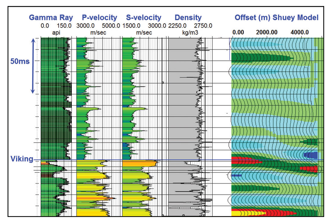
The value oriented quality control effort can be pursued in map view as above, but can also be evaluated by viewing the gathers themselves, in particular at gathers that tie important well control data. To illustrate this assertion, we chose a deep well that is a good Viking producer and was logged with a full log suite including dipole measurements. This well was used to create a 0 to 34 degree Shuey (1985) AVO model representing the correct AVO response. The logs and Shuey AVO model are illustrated in Figure 3. The Viking reservoir is a shoreface sandstone of less than 10m thickness. Its coarsening upwards profile is evident on the Gamma Ray log. The Viking has up to 14% porosity, which is quite apparent in the bulk density logs. The sandstone has a very low Vp/Vs ratio, which gives rise to its AVO behavior. The Viking peak undergoes a clear Type II AVO response, which we expect to see in the real data if the phase, resolution, noise attenuation, and amplitude fidelity are all handled correctly and in an AVO preserving fashion in the processing.

At every major step in the processing sequence, we create a 3x3 supergather at the well location for AVO analysis. Each super-gather has final velocities, statics and optimal phase rotation applied. The AVO response of the gather is compared to the synthetic “answer” in a qualitative and a quantitative fashion. This process is carried out at 15 major processing steps, and is informative of the effect associated with each processing step. In this sense we isolate and evaluate the relative and combined importance of each step in the processing sequence. These analysis steps include the first geometry sort of the data, the first surface-consistent deconvolution, the first surface-consistent scaling, the second surface-consistent deconvolution, each major noise attenuation step, the application of the unbiased surface-consistent scaling, and before and after interpolation and pre-stack migration.

In performing this analysis, we encountered several uncomfortable and challenging problems. At each step in the processing sequence, a single scalar was calculated and applied to the gather. This needed to be done so that the gathers from each step in processing could be meaningfully compared. The reference AVO model was also scaled to match the overall amplitudes in the final unbiased interpolated and pre-stack imaged gather. There is little doubt that the choice of scaling has some effect on the relative comparability of each gather, and likely contributes to the close match of the final product to the synthetic. The phase of each gather was also important in this comparison. We also made a series of phase corrections to the gathers so that the comparison could be as objective and consistent as possible. This correction was made by tying each gather to the synthetic model, and was carried out at each point in the processing wherein the phase was expected to materially change. As with the scalar, a single phase shift was applied to the entire gather. The key phase analysis and application steps were:

• On the Raw data
• After Q-compensation
• After the first surface consistent deconvolution
• After the second surface consistent deconvolution
• After pre-stack imaging

The extraction windows for the Viking peak AVO amplitudes were also updated for each of these stages.

With these corrections applied, we compared the gathers through the major steps in the processing sequence. We compared a total of 15 different processing versions of the gather at the reference well with the reference synthetic. Figure 4 illustrates a subset of those gather comparisons. The gathers shown are supergathers, with offsets increasing to the right. The Viking peak is identified by a yellow arrow. Figure 4(a) is the reference Shuey synthetic at a comparable scale and offset step as the real data gathers. Figure 4(b) is the raw gather and is mostly dominated by groundroll. Although nearly drowned by the groundroll amplitudes, the Type II AVO effect on the Viking peak remains visually observable. Figure 4(c) has Q-compensation and groundroll suppression. Figure 4(d) has the first pass of surface consistent deconvolution and scaling. The noise in the data is now more prevalent at higher frequencies. Figure 4(e) has FXY noise attenuation and abnormal amplitude removal. Figure 4(f) has the second pass of surface consistent deconvolution, surface consistent scaling, and FXY deconvolution. Figure 4(g) is the pre-stack time migrated gather. Figure 4(h) is the final interpolated pre-stack time migrated gather. Throughout this progression of processes, the Type II AVO behavior at the Viking level remains visually observable. The goal of processing is to reveal the AVO effects inherent in the seismic experiment, not to create the AVO effects themselves. As such, we had hoped that our VOQC approach would identify the Viking AVO behavior from start to finish; and it did.

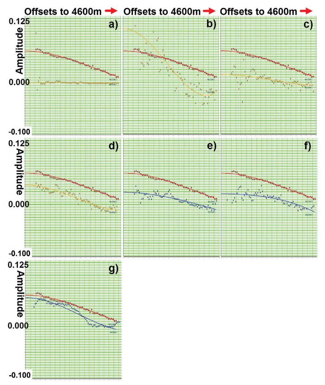
The question remained as to how accurately the processing would reveal the AVO of the Viking. To be specific, we wanted to know how accurately our estimate of the AVO characteristics of the Viking would be at each stage in the processing. The changes in AVO accuracy would inform us of the value of each step in the processing relative to this single control point. The question of accuracy was answered through comparing modeled AVO curves extracted from the data. This AVO modeling of each gather is equivalent to industry-standard AVO inversion computations. Figure 5 illustrates the modeled AVO curve extractions of intercept and gradient for the same gather as previously shown in Figure 4. In each case, the synthetic data are given as red data points with a red curve. The real data are represented by orange points and curve for the first 4 gathers, and then by blue points for the rest of the gathers. Figure 5(a) is the AVO response for the raw gather. The groundroll amplitudes truly swamp or act to obscure the AVO characteristics of the Viking peak. Figure 5(b) is the AVO response for the Q-compensation and groundroll suppression. Figure 5(c) is the AVO response for the first pass of surface consistent deconvolution and scaling. Figure 5(d) is the AVO response for the FXY noise attenuation and abnormal amplitude removal. Figure 5(e) is the AVO response for the second pass of surface consistent deconvolution, surface consistent scaling, and FXY deconvolution. Figure 5(f) is the AVO response for the pre-stack time migrated gather. Figure 5(g) is the AVO response for the final interpolated pre-stack time migrated gather. Resolution enhancement is crucially important to most targets in the WCSB, however, it can be seen that each resolution enhancement step increases the noise in the AVO extraction. This is shown in Figures 5(b) and 5(c). The interpolation-pre-stack imaging step of Figure 5(g) has a less scattered or noisy appearance than that of the uninterpolated imaging step of Figure 5(f).

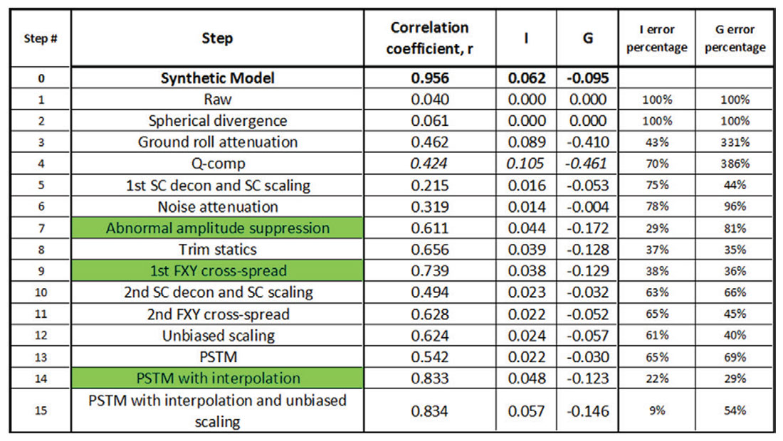
We can further compare the AVO extractions by reference to the estimated intercept and gradient for each step in the processing sequence, and compare those values to the intercept and gradient seen in the reference Shuey synthetic. The scaling that we applied to each gather is of critical importance to the validity of this comparison, and may be a subject of further discussion. We also kept track of the correlation coefficient of the Shuey AVO curve fit for each step of the processing. The correlation coefficient is an important addition to the analysis since it is unaffected by any potentially unsatisfactory dc-shift issues with the scaling (Rodgers and Nicewander, 1988). Figure 6 gives the correlation coefficient, r, the intercept, I, and the gradient, G, for all 15 processing steps. There is a general progression to closer matches of intercept and gradient the further along the processing sequence we progress. The correlation coefficients also tended to increase as the processing sequence progressed, although the values always dropped immediately following resolution enhancement. Three steps are colored green as an identifier of large improvements in the correlation coefficients.

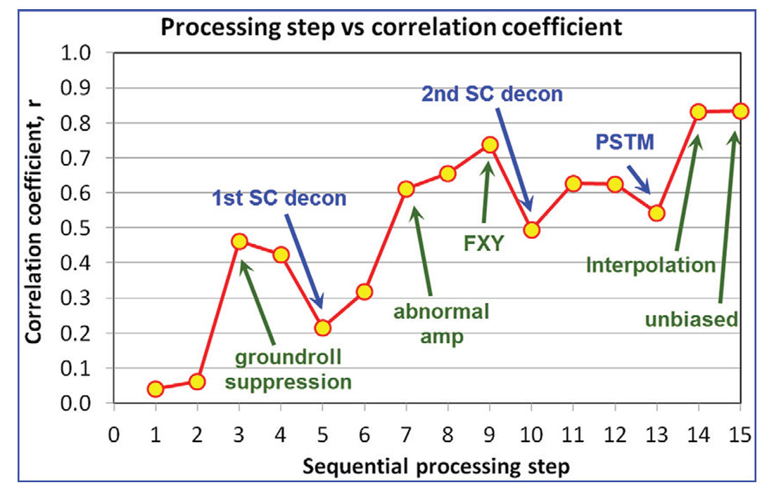
The changes in the correlation coefficient throughout the processing sequence appeared to be largely due to changes in the amount of noise in the gathers rather than due to alterations in the AVO characteristics of the data. As such, the changes in correlation coefficient represent the trade-off between resolution and noise that are commonly of concern during processing. This gather VOQC example is thus very supportive of the value of AVO preserving noise reduction processes. Figure 7 is a chart of the correlation coefficient versus processing step. The sequence numbers match those of Figure 6. The unbiased surface consistent scaling method had very little, if any, impact on the AVO fidelity at this single gather, which stands in contrast to its long-wavelength effect as seen on the VOQC map evaluation performed earlier.

Discussion

The practicality of carrying out similar work to that of our case study example may be debated by some. There is little doubt that the phase and scaling issues that we encountered do require further thought. Our approach of applying single constant phase corrections and amplitude scalers to the gathers at each stage of the processing did leave some dc-like amplitude differences in the data, and could be replaced by some other practical methodology. Nevertheless, we were able to produce coherent results without an undue effort despite the fact that we had never attempted such a quality control effort before and had never seen such an effort in the literature. Given the importance of AVO work in our business today, we believe that efforts similar to ours will become more commonplace, and that best practices for how to carry them out will evolve quickly.

The AVO analysis on gathers did show some important changes in amplitude behavior that could not have been impacted by the phase corrections and amplitude scalars. Of most interest was the decrease in correlation after every resolution enhancement stage. Despite the hypothesis we offered regarding the noise being brought up by these processes, this effect should be followed up by further work. Paul Anderson (personal communication) suggested to me that he had qualitatively observed this effect before. Given the importance that tuning has for AVO analysis (Hamlyn, 2014), and therefore our general need to improve resolution for AVO, many of us will continue to wrestle with this phenomena in the future.

The importance of carrying out a study on a single well or a set of wells for AVO-centric targets cannot be overstated. At the same time, quality control carried out in a map sense is equally important. Certain long wavelength phase and amplitude effects within the data, such as the unbiased versus biased scaling shown in our case study, may be entirely missed when viewing a single well. In the study of the unbiased surface consistent scaling method, the map analysis showed an improvement in the accuracy of the amplitudes for the Viking and the Wabamun zones. This improvement had a long wavelength characteristic. Certain noise and imaging effects also may be more or less likely to be illustrated in either the gather domain or on maps. If the VOQC quality control methods lack sufficient comprehensiveness, the usefulness (or limitation) of the process may be missed.

Conclusions

The VOQC method is an additional quality control effort that should be done through an integrated effort between processors and interpreters. This method keeps the end use of the data in mind at all times, and thus has a bearing on the economic target of any work. VOQC will occasionally require a control experiment to determine the potential value of a process, but will always require that some quality control effort be continuously directed to the target zone in the data. In an economic paradigm that is increasingly concerned with AVO and even azimuthal studies, VOQC suggests that targeted attention be paid to AVO and azimuthal effects throughout the processing project. We argue that the VOQC concept should be increasingly undertaken by processors and interpreters who wish to test the reliability, relevance, and value of their efforts. Such VOQC tests should be useful in directing seismic efforts to their greatest use. The unbiased surface consistent scaling method of Cary and Nagarajappa (2013a, b) could only be objectively proven to be superior through a VOQC map analysis approach; all other efforts led to subjective results. And this is the main point of this work: that the value of superior processing is best shown by tests that consider the economic impact of the processing.

Acknowledgements

The data used in this study was licensed from an undisclosed data owner, and the work was shown with permission of Santonia Energy and the data licensor. This work was originally shown to an audience of about 300 persons, and in greater detail, on March 4, 2014 at the 2014 CSEG Symposium.