Summary
Knowledge of formation pore pressure is not only essential for safe and cost-effective drilling of wells, but is also critical for assessing exploration risk factors including the migration of formation fluids and seal integrity. Usually, pre-drill estimates of pore pressure are derived from surface seismic data by first estimating seismic velocities and then utilizing velocity-to-effective stress transforms appropriate for a given area combined with an estimated overburden stress to obtain pore pressure. So, the accuracy of velocity models used for pore pressure determination is of paramount importance. This paper briefly discusses some of the causes and mechanisms of overpressures, and then reviews the available methods of velocity model building, mentioning therein the shortcomings and/or the advantages of each.
Introduction
An understanding of the rock/fluid characteristics of subsurface formations is of critical importance in the evolution of oil and gas fields. During the exploration phase, pore pressure prediction for example helps in studying the hydrocarbon trap seals, mapping of hydrocarbon migration pathways, analyzing trap configurations and basin geometry and providing calibrations for basin modeling. Predrill pore pressure prediction allows for appropriate mud weight to be selected and drill casing program to be optimised, thereby enabling safe and economic subsurface drilling. The importance of determination of this information has gradually been realized as some major well disasters have led to the loss of precious human life, material and adverse publicity. It is time now that pore pressure prediction formed an integral part of prospect evaluation and well planning.
Besides drilling a well, the only way to predict potential hazards like overpressured subsurface zones is through the use of seismic surveys. Although such an analysis originated with the work of Terzaghi (1930) ( a soil scientist), it was the works of Hottman and Johnson (1965) (both petrophysicists) and Pennebaker (1968) (drilling engineer), that drew the attention of geoscientists. While a range of disciplines are involved and needed in a comprehensive pore pressure analysis, geophysicists play a key role in many ways (Bruce, 2002). Seismic methods detect changes of interval velocities with depth from velocity analysis of CMP data, and so geophysicists are involved in seismic interpretation and determination of rock properties which are related with pore pressure (Bell, 2002). Over pressured formations exhibit several of the following properties when compared with a normally pressured section at the same depth (Dutta, 2002): (1) higher porosities (2) lower bulk densities (3) lower effective stresses (4) higher temperatures (5) lower interval velocities (6) higher Poisson’s ratios.
Seismic interval velocities get influenced by changes in each of these properties and this is exhibited in terms of reflection amplitudes in seismic surveys. Consequently, velocity determination is the key to pore pressure prediction.
Some definitions
A detailed description of pore pressure terminology can be found in Bruce and Bowers (2002), Bowers (2002) and Dutta (2002). We include some of these definitions here for convenience.
During burial, normally pressured formations are able to maintain hydraulic communication with the surface. Pore pressure or formation pressure is defined as the pressure acting on the fluids in the pore space of a formation. So, this pore fluid pressure equals the hydrostatic pressure of a column of formation water extending to the surface and is also commonly termed as normal pressure. Fig.1 illustrates such a subsurface condition. Hydrostatic pressure is controlled by the density of the fluid saturating the formation. As the pore water becomes saline, or other dissolved solids are added, the hydrostatic pressure gradient will increase.

Also, sonic velocity, density and resistivity of a normally pressured formation will generally increase with depth of burial and the way such rock properties vary with burial under normal pore pressure conditions is termed its normal compaction trend.
Pore pressure gradient is defined as the ratio of the formation pressure to the depth and is usually displayed in units of psi/ft or equivalent mud weight units in pounds per gallon (ppg).
Overburden pressure at any depth is the pressure that results from the combined weight of the rock matrix and the fluids in the pore space overlying the formation of interest. Overburden pressure increases with depth and is also called the vertical stress.
Effective pressure is defined as the pressure acting on the solid rock framework. Terzaghi defined it as the difference between the overburden pressure and the pore pressure.
Effective pressure thus controls the compaction that takes place in porous granular media including sedimentary rocks and this has been confirmed by laboratory studies (Tosaya, 1982; Dvorkin (1999)). Any process or condition causing a reduction of effective stress will result in overpressure. In overpressures, the pore fluids bear part of the weight of the overlying rocks. A lower effective stress and a higher porosity tend to lower the rock velocity. Consequently, a relationship between velocity and effective stress, porosity and lithology could be used to study pore pressures.
Causes of overpressure
Overpressures in sedimentary basins have been attributed to different mechanisms but the main ones are related to increase in stress and in-situ fluid generating mechanisms. The ability of each of these processes to generate overpressures depends on the rock and fluid properties of the sedimentary rocks and their rate of change under the normal range of basin conditions.
Increase in stress: During deposition of sediments, with the increase in vertical stress, the pore fluids escape as the pore spaces try to compact. If a layer of low permeability, e.g. clay, prevents the escape of pore fluids at rates sufficient to keep up with the rate of increase in vertical stress, the pore fluid begins to carry a large part of the load and pore-fluid pressure will increase. This process is referred to as undercompaction or compaction disequilibrium (Hubbert and Rubey, 1959), and is by far the most well understood overpressure mechanism used to explain and quantify overpressures in Tertiary basins where rapid deposition and subsidence occur, e.g. the Mississippi, Ornico and Niger Delta regions (Yassir and Addis, 2002).
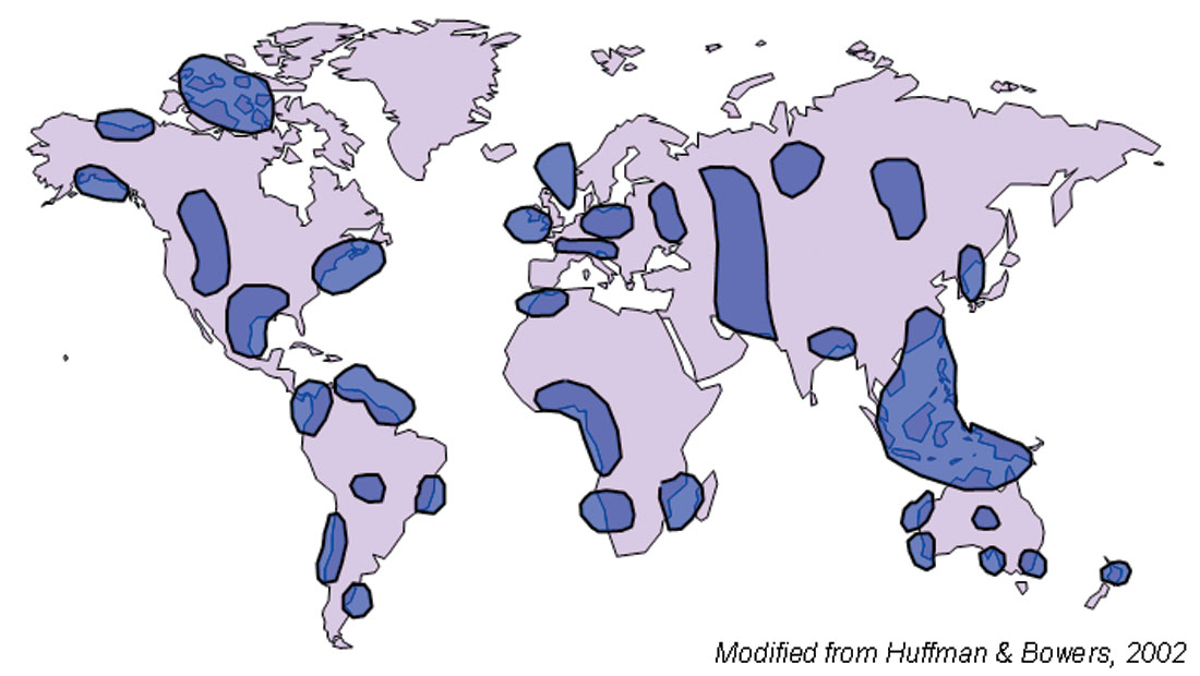
Tectonic subsidence or overthrusting can also result in an effect similar to undercompaction in that the increased vertical stress is taken up by the pore fluids and reflected as enhanced pore pressures (Dutta, 1987). Some notable occurrences of over pressuring and present day compressional tectonics include the Barbados Accretionary Prism (Trinidad), the Andes, Papua New Guinea, California and Gulf of Alaska. Fig. 2 shows a schematic map of global overpressure occurrences.
Secondary Pressure Mechanisms: A second class of pressure mechanisms have been grouped together under the heading of secondary pressure mechanisms because they occur on top of primary compaction and undercompaction processes. These mechanisms are also called unloading mechanisms because they tend to cause the in-situ pore pressure to increase at a fixed overburden, which results in a decrease in the effective stress on the matrix, hence the term unloading. The basis for the unloading concept comes from the rock mechanics literature where the role of effective stress on compaction of porous granular media has been studied for over 50 years. As noted in figure 1, unloading is identified by the reduction in effective stress as the pore pressure increases rapidly under specific conditions.
Fluid Expansion Unloading Mechanisms: Over pressure in the pore spaces of a formation can result by fluid expansion mechanisms as the rock matrix constrains the increased volume of the pore fluid. These include processes like heating, clay dehydration (Dutta, 1987), hydrocarbon maturation (source rock to oil and gas), etc. Of these mechanisms, the two that are most significant in real rocks are clay diagenesis and hydrocarbon maturation. In particular, hydrocarbon maturation is the most dangerous mechanism because it generates fluid pressures that locally exceed the fracture strength of the rocks as the hydrocarbon fluids fracture out of the source interval to migrate to lower pressure environments.
Lateral transfer: A fluid-expansion type of mechanism can also result when sediments under any given compaction condition has fluid injected into it from a more highly-pressured zone (Fertl, 1976). This could happen when migration of fluid along faults takes place or if a high-permeability pathway such as a reservoir, or a connected network of reservoirs and faults allows transmission of pore fluid from a deeper trap to a shallower one, a process termed lateral transfer.
Structural Uplift: A very dangerous form of unloading occurs when sediments are uplifted by tectonic activity. Uplift of sediments alone will not cause unloading if the overburden load is not changed, but when the overburden is reduced during uplift either by syn-depositional tectonic processes or by erosion, the accompanying reduction in overburden results in the original in-situ pore pressure being contained by a much lower overburden, which results in a reduction of the effective stress, and unloading.
For more details on overpressure generation in sedimentary basins, the reader is referred to Osborne and Swarbrick (1997) and Huffman (2002).
Detection of Overpressures
The methods currently being used for detection of overpressures exploit the deviation of formation properties from an expected or normal trend in the area of interest. Well logs provide the most extensively used and a reliable means to construct trends and detect overpressures. Usually, density, resistivity and sonic velocity data either continue to increase or remain constant after they depart from their normal trends. However, this information is forthcoming only after the well has been drilled. Detection of overpressures before drilling is more useful as precautions can be taken and planning can be done accordingly. Reflection seismic methods are commonly used for this purpose and exploit the fact that overpressured intervals have lower velocities and impedances that are lower than normally pressured intervals at the same depth.
Empirical relationships
As porosity is a direct measure of compaction, Athy (1930) put forward the following exponential relationship between porosity and depth
φ(z) = φ0e−cz
where φ(z) is porosity at depth, φ0 is the porosity at z=0 and c is a constant.
Since then other modifications have been suggested to this model and this equation has been recast into (Dutta 2002),
φ(z) = φ0e−κσ
Terzaghi’s equation is given as follows
φ(z) = 1 - φ0σc/4.606
and there are other empirical relationships as well.
One of these relationships is used to compute the effective stress from the porosity and then the pore pressure is computed easily from Terzaghi’s relationship
S = P + σ
S = vertical overburden stress
P = pore fluid stress
σ = effective stress acting on the rock frame.
The commonly used approach for relating acoustic interval velocity to pore pressure is the Eaton’s empirical method (Eaton, 1968, 1972).
According to Eaton

where
Pp = Predicted (shale) pore pressure
Pobs = Overburden pressure (rocks and fluids)
Phyd = Hydrostatic pressure (fluids)
Vi = Interval velocity (seismic data)
Vn = Normally compacted shale velocity
Pp, Phyd and Vn are empirically derived values from relevant well data and the interval velocity is derived from seismic processing. The Eaton method has been described as a “horizontal” pressure method because it compares an in-situ physical property to a “normally-compacted” equivalent physical property at the same depth. This implies that the method is valid as long as the normal compaction trend can be constructed for all depths of interest. For high sedimentation rates as is common in Gulf of Mexico slope and deepwater environments, the normal compaction trends are absent. From a practical perspective, the Eaton trend line must often be adjusted from one location to another to handle local variations, which can become rather “non-physical” in its implementation. This makes the application of the Eaton equation for large seismic volumes with thousands to millions of traces very difficult to implement.
The Bowers Method
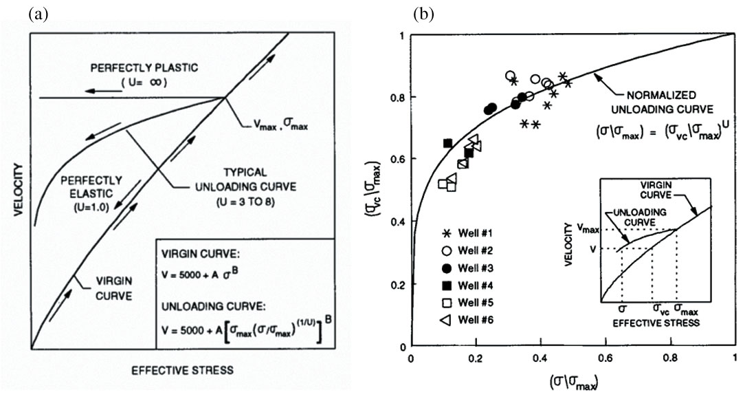
As effective stress methods became more prevalent, experts in the geopressure community began seeking more robust equations that had a physical basis in the compaction process and could be modeled in the laboratory. In a seminal paper on the subject, Bowers (1994) published a new power law equation that allowed normal compaction, undercompaction and unloading to be handled by a single equation that could be calibrated to existing data even in cases where no normal compaction trend is present (e.g. deepwater settings). Bowers recognized the fundamental concept that unloading intervals are effectively zones of stress hysteresis where the effective stress drops and is maintained at a lower level until some event causes the pore pressures to bleed off. This equation (figure 3a) allows the user to define the normal compaction trend for an area by defining a Vo term and a coefficient and exponent for the effective stress. In unloaded intervals, the equation requires that the maximum stress state where the unloading started be known, and the unloading trajectory is then defined by an unloading exponent that is fit to the offset well data (figure 3b). In the case where the unloading exponent equals unity, the stress ratio term in the expanded equation collapses back to the equation for the normal compaction trend or virgin curve as Bowers called it.
Overpressure detection from borehole data
Changes in pore pressure can be recognized on regular formation evaluation tools such as sonic, resistivity, porosity and density logs. These logs show the effects of pore pressure because of the relationship between compaction, porosity, density and the electrical and acoustic properties of sediments. As a rock compacts, the porosity is reduced and the density increases, which also causes the bulk modulus and shear modulus to also increase because of increases in grain contact area and grain contact stress. This process continues until the mechanical process of compaction is slowed by either the stiffness of the rock frame or by increases in pore pressure that resist further compaction. In cases where the sealing rocks allow fluid pressures to counteract the vertical stress and undercompaction occurs, the result of this process is to slow down the decrease of porosity and increase in velocity and density, but NOT to stop it totally. As such, undercompacted intervals will still follow the normal compaction pathway but the rocks in such a condition will show higher porosities and lower velocities than a normally compacted rock at the same depth of burial. This effect can be seen on log displays as shown in figure 4.
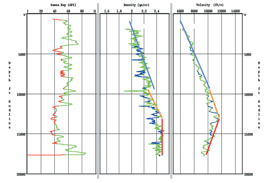
When unloading pressure mechanisms occur in the subsurface, the increase in fluid pressure causes the compaction process to stop, which causes the porosity and density to cease changing with depth of burial. As the fluid pressure increases and the effective stress drops, the rock is not able to increase its porosity because the compaction process is irreversible. Therefore, the grain contact area also is essentially unchanged. However, the increase in the pore pressure does cause a reduction in the grain contact stress, which causes the velocity to drop. This produces the classic signature of unloading as shown in figure 4 in the deeper section where the density log ceases changing and the sonic log undergoes a sharp reversal. This effect can be recognized very easily by cross-plotting sonic and density logs for a well as shown in figure 5. In such plots, the unloaded zone becomes very obvious because of the abrupt change in the velocity density plot as the velocity drops and the density stays the same.

VSP data: Zero offset vertical seismic profiles can be used for detection of high pressure zones in the subsurface ahead of the drill bit using seismic inversion methods. Figure 6 shows a pseudo interval velocity trace in well A - 1 from eastern India. The inversion was done using the procedure outlined by Lindseth (1979). A well about 1.5 km away from A-1 had encountered a blowout at 2100 m. Being adjacent, high pressure was expected in this well also at around the same depth. VSP data were acquired in this well and the pseudo interval velocity trace generated from the corridor stack trace. As is evident from the ‘knee’ (Fig.3), high pressure was predicted at 2930 m. However, due to some practical difficulties, drilling for this well was suspended at 2650 m, and up to that depth no high pressure zones were encountered.

Another well A-2, about 2 km away from A-1 was drilled (depth not available) and VSP data was acquired and processed. The ‘knee’ seen on the pseudo interval velocity trace indicated that high pressure was to be expected at 3200 m. Drilling was continued further and high pressure was encountered at 3180 m in accordance with the prediction. At the time this work was done, pressure indications were read off from the interval velocity traces
Overpressure detection from seismic data
The estimation of pore pressures from seismic data uses seismically-derived velocities to infer the subsurface formation pore pressure. The Eaton method uses a direct transform from velocity to pore pressure, while the Bowers method estimates the effective stress from the velocities and then calculates the pore pressure. There are many different types of seismic velocities, but only those velocities that are dense and accurate and are close to the formation velocity under consideration, will be of interest. The following methods have been used with varying degrees of success and will be discussed individually.
- Dense velocity analysis.
- Geologically consistent velocity analysis.
- Horizon-keyed velocity analysis.
- Automated velocity analysis.
- Velocity determination using reflection tomography.
- Residual velocity analysis.
- Velocities from seismic inversion.
Before discussing these methods, something must be said about data conditioning for geopressure.
Data Conditioning
Velocity analysis for geopressure prediction requires a level of detail in the velocity analysis that goes beyond the normal stacking velocity approaches used for traditional imaging work. Imaging velocity analysis usually results in a highly smoothed velocity field that is designed to operate with migration algorithms that are not designed to handle abrupt changes in the velocity across features like faults, salt bodies and other geological features. Unlike imaging velocity analysis, velocity analysis for geopressure prediction is designed to detect such abrupt velocity changes and record them for use in the prediction process. To facilitate this process, seismic gathers are usually conditioned for geopressure prediction to assure the highest quality velocity analysis possible.
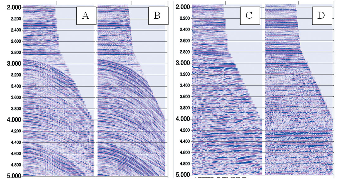
Atypical data conditioning process for geopressure prediction usually includes a band-pass filter to remove high frequency noise that degrades semblance responses, plus processes like Radon noise suppression and other pre-stack noise suppression techniques. The goal of these processes is to improve the quality of the semblances to enable more robust picking. These processes are usually applied to pre-stack time-migrated gathers, or pre-stack depth migrated common image point (CIP) gathers. Some advanced processes like wavefield reconstruction are also applied for data conditioning in extreme conditions. Figure 7 shows an example of such a reconstruction process where aliased gathers are reconstructed to allow a demultiple algorithm to work better. The application of such techniques can dramatically improve the quality of the resulting velocity analysis.
1. Dense velocity analysis
Velocity information is determined from seismic measurements of the variation of reflection time with offset, i.e. CDP gathers. It is the hyperbolic characteristic of these reflection time-offset curves which forms the basis for computation of velocity analysis. A statistical measure of trace to trace similarity (cross-correlation or semblance) is employed to determine resulting amplitudes which are posted on a spectral display.
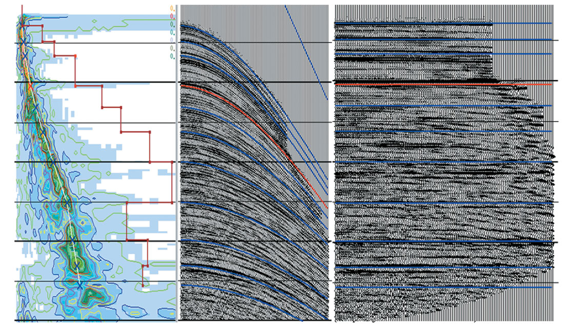
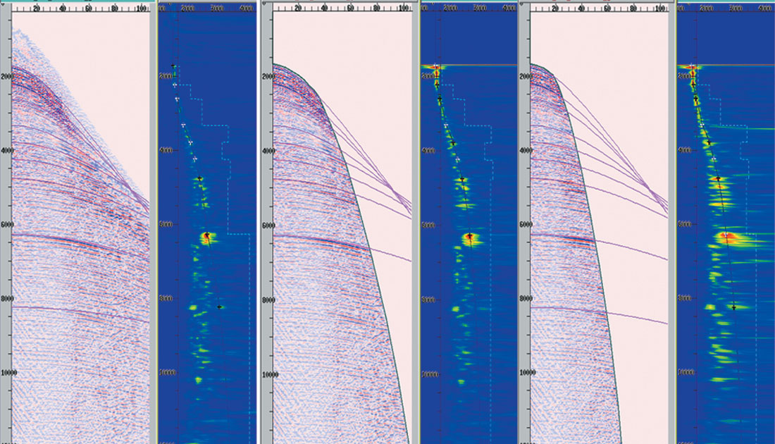
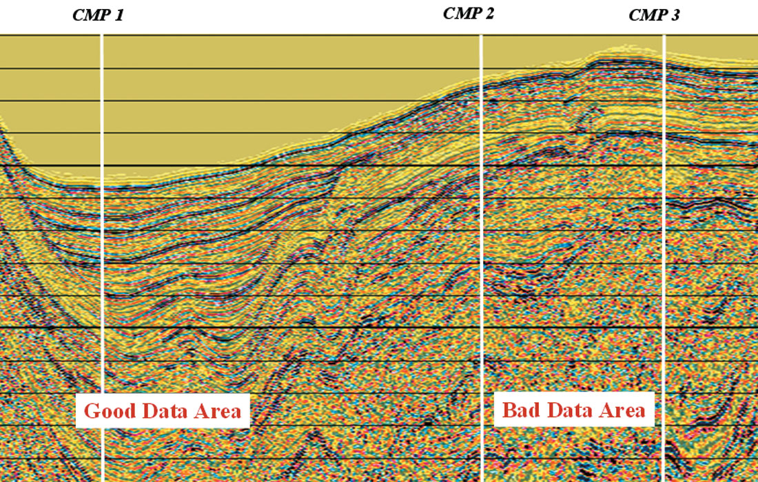
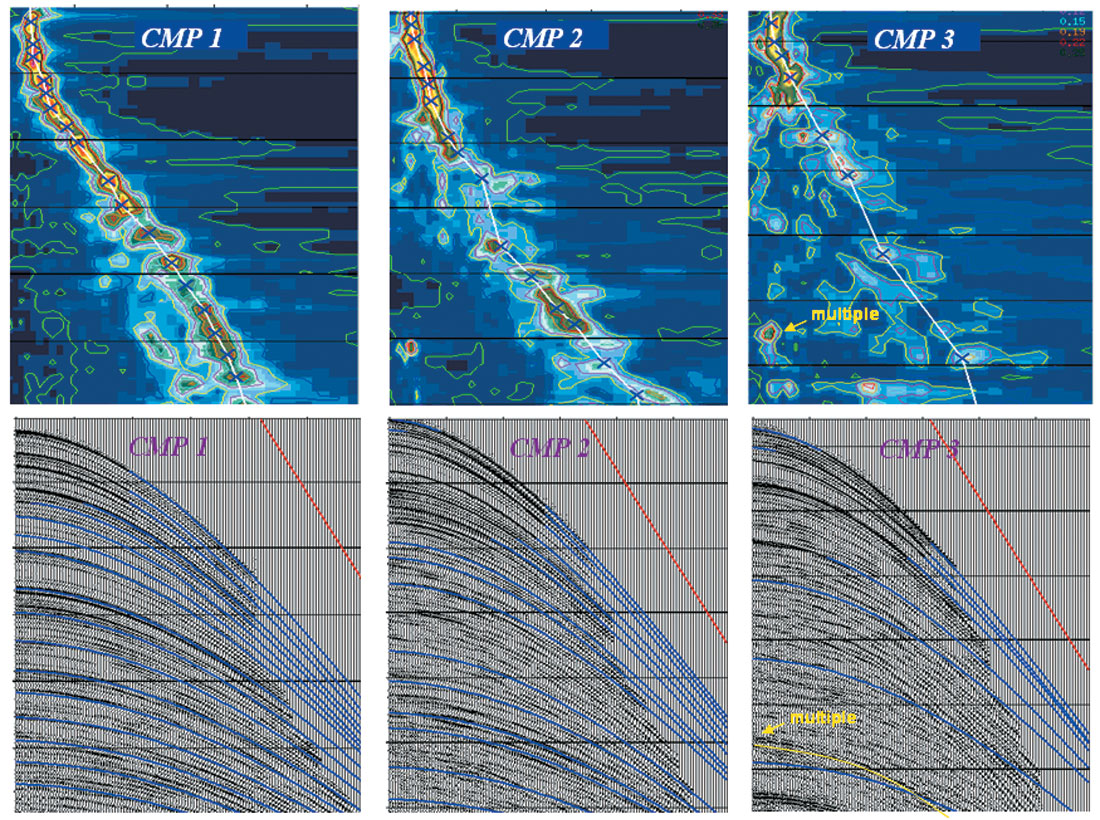
Figure 8 shows traditional velocity analysis carried out using semblance analysis along hyperbolic search on a CDP gather. Individual velocity picks are marked on the display keeping in mind the energy maxima and connecting all the primary energy peaks yields the RMS velocity function (white line) and its calculated interval velocity (red line) derived using the Dix equation. Computing interval velocities from stacking velocities can often be inadequate as Dix’s equation assumes flat layers of uniform velocity. For geopressure prediction, the goal is to pick velocities to optimally flatten the data (figure 9). It is often observed that basic processes such as how the data are muted can improve or degrade the semblance picking process (figure 10). The biggest difference in velocity analysis for geopressure prediction is that surface like faults, which are usually ignored in traditional velocity analysis due to the absence of semblance events at the fault surface, are actually picked to assure that velocity changes across the fault are honored. It is also often observed that the quality of velocity analysis is directly affected by the quality of the underlying imaging. Figure 11 shows an example of 3 CDP’s on a seismic line with variable data quality. This example shows how significant the image quality is for good velocity analysis.

Example 1
Traditional stacking velocities have been used to construct pressure prediction cubes that provide new insights into the 3D subsurface pressure distribution. Figure 12 (a) shows a cross-section through a final velocity volume from the Columbus Basin, offshore Trinidad & Tobago (Snijder et al., 2002). An interval velocity cube was first generated from DMO velocity functions and DMO velocities slices generated along 150 ms thick time slices parallel to the sea bed. Next, the DMO velocities were converted into interval velocities using Dix formula and smoothed using a 3000m running average filter. These smooth interval velocity slices were used to convert the time slices into depth and generate the seismic interval velocity cube with respect to depth. The horizons tracked on the seismic time volume were converted to depth using the smoothed velocity function and overlayed on the interval velocity depth volume. The rather large mismatches between this modelled velocity and well data were minimized by applying the first-order laterally variable velocity correction map to the velocity cube.
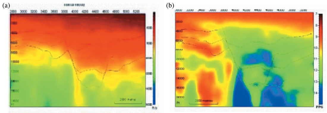
Actual measurements carried out in wells like RFT, MDT and mud weights etc. were next used to perform a final calibration of predicted pressure to actual pressures via cross-plots. A consistent bias found was removed by using a simple linear correction.
Figure 12(b) shows a cross-section through the calibrated pore pressure gradient volume. More details about the method and its implementation can be picked up from the reference cited above.
Example 2
This example is from the Macuspana Basin, located at the north of the Montagua-Polochic fault system in South Mexico (Caudron et al., 2003). Complex shale tectonics has complicated the basin’s geological structure setting and presents a challenge for petroleum exploration and production. Drilling in the area has confirmed compartmentalization of pore pressures, which is associated with the complex structure.
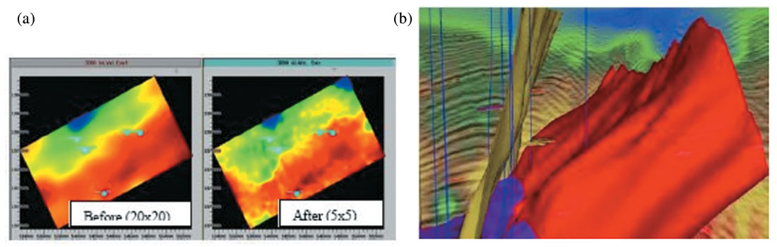
RMS velocity functions were picked on a grid of 20 x 20 (inlines x crosslines) for use in 3D prestack time migrated gathers. The quality of the seismic data and the complex nature of the structures being investigated suggested manual residual moveout picking so as to refine the RMS velocity to a grid of 5 x 5 (150m x 150m). Next, the velocity field was calibrated with well log data.
Figure 13(a) shows a comparison of an interval velocity map at a depth of 3000 m before and after the velocity refinement and calibration. Clearly, more detailed velocity changes can be seen on the refined interval velocity map.
Figure 13(b) shows the pore pressure overlaying the seismic data. The growth fault in red and the fault in yellow on the display appear to be pressure boundaries. Apparently, the high compartmentalized pressure distribution has been influenced by the pattern of the fault system. The growth faults might have prevented the expulsion of water from the pores of sediments during compaction and diagenesis.
2. Geologically consistent velocity analysis
Traditional stacking velocities, while producing good quality stacks usually do not follow key geologic features like faults, lithologic boundaries and major sequence events in a consistent fashion. Geologically-consistent velocity analysis addresses these shortcomings and can also utilize well logs to choose key surfaces for the picking of the velocities. Seismic time horizons are first interpreted on a preliminary stacked volume. The well control in the area is combined with these horizons to produce an initial interval velocity field. This regional velocity field is superimposed on the displays. The processor now picks the velocities at several locations along the line, changing the model wherever necessary. The velocities are picked as interval velocities and converted into stacking velocities. Such a velocity model, when properly designed, will honor both the seismic data and the well control.
Figure 14 shows a comparison of traditional and geologically consistent velocities. The sonic well log in time (blue) is overlain on the velocity curves (red). Note that while the traditional velocities yield a ‘smoothed’ approximation to the well log, the geologic velocities follow the detail of the geologic layers, i.e. the changes in the velocity on the sonic log are followed much more closely.
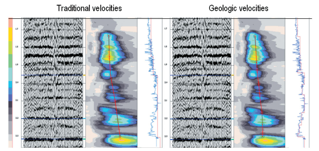
Figure 15 (a) and (b) illustrates how the use of geologically consistent velocities has improved the accuracy and provided greater spatial consistency in comparison to the more traditional way of picking velocities.

In the traditional approach, the 3D velocity field is generated by interpolating within the picked velocity functions. This can lead to ‘bull’s’ eyes in the interval velocity maps generated for QC. Also, for thin layers, a small variation in the RMS velocity picking causes a large change in the interval velocity. These problems are addressed by smoothing the velocity field significantly. Such a severe smoothing often smooths out some of the subtle and real velocity variations along with the noise.
Thus the geological approach to velocities ensures that the geologically consistent velocities are horizon consistent, laterally consistent and so ensures bull’s eyes are avoided and realistic values that tie to the wells at each line intersection are consistent. While these velocities are geologically more meaningful and correct, they need to be used carefully. Another point that needs mention here is that such a velocity field may not properly flatten the gathers. If this is an issue in the area of interest, then an alternative method would need to be explored. Geologically consistent approach to velocity analysis is sometimes augmented with spatial modeling (geostatistics).
3. Horizon-keyed velocity analysis (HVA)
Traditional velocity analysis provides the velocity functions along the seismic profiles at selected points. Even for cases where the S/N ratio is above moderate and the structure is not complex, the accuracy is not sufficient for computation of reliable interval velocities, depth sections and for getting good quality migrations.
Horizon velocity analysis (HVA) provides velocities at every CDP location along the profile (Yilmaz, 2001). The velocity analysis is computed for a small number of time gates centered on normal incidence travel times that track given reflection horizons. Since only a few time gates are to be considered and the range of trial velocities is limited, the computer time is used in a better way in conducting an intensive analysis on important events, than on time zones between horizons.
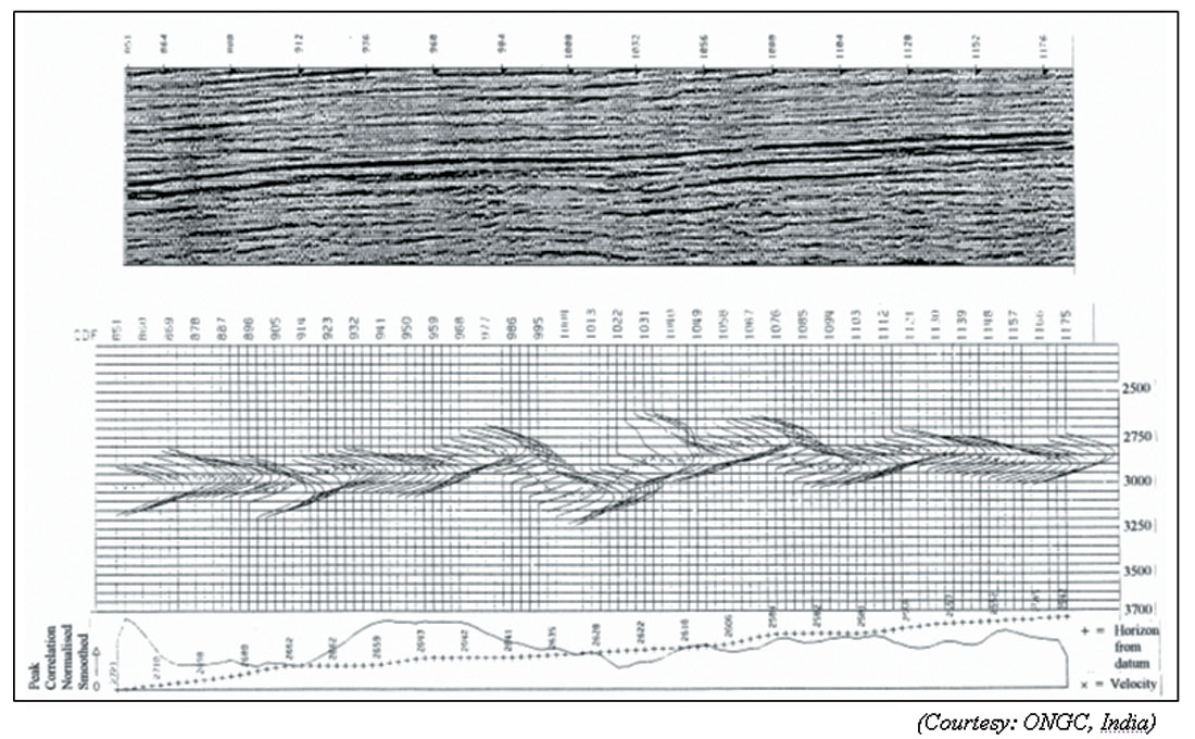
Figure 16 shows a reflecting horizon and its associated computed HVA. Once HVA computation is completed for the main horizons in the section, it is possible to build up a grid by computing the interval velocity between these main horizons.
Horizon velocity analysis can provide high spatial resolution but the temporal resolution may be low for pore pressure prediction applications. Due to this reason, this approach should be applied in conjunction with another technique where this information proves useful.
4. Automated velocity inversion
An automated velocity inversion technique has been proposed by Mao et al., 2000 in which stacking velocities are assumed equivalent to RMS velocities, an assumption that would require appropriate corrections for reflector dip, non-hyperbolic moveout and event timing. Such assumptions can only be satisfied with prestack depth migration as demonstrated by Deregowski 1990. The data input to this method are migrated image gathers. The method comprises a series of algorithmic components:
- As the first step, reflection events in 3D space are first analysed. Those events and their corresponding stacking velocities that exhibit maximum spatial consistency are picked.
- Next, treating the stacking velocities as RMS velocities and using a least-squares optimisation procedure constrained interval velocities are computed.
- These velocities are then smoothed using a cascaded median filter, keeping in mind the desired resolution limits in terms of the magnitude and the lateral extent of the smallest velocity anomaly to be resolved.
The method yields a 3D velocity model in which steep dips and relatively rapid velocity variations have been handled (Mao et al., 2003).
Banik et al., 2003 demonstrate the application of such a velocity procedure to a pore pressure system in a deep-water basin, offshore West Africa. Due to the sharp lateral changes in velocity in this area and the absence of deep-water wells, instead of the empirical methods (e.g. Eaton’s equation), a proprietary velocity to pore pressure transform was used. Figure 17(a) shows a PSTM seismic section along a dip line. Figure 17(b) shows the high resolution velocity (m/s) for the line in Figure 17(a).
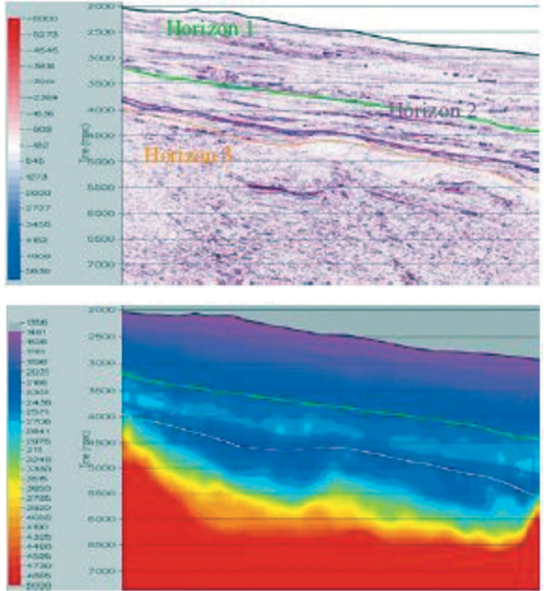
Figure 18 shows the computed pore pressure for Figure 17. The pressure gradient is seen to increase slowly and gradually in the shallow portion but beyond a prominent geologic horizon, it increases rapidly, before reversing back to a lower value.

5. Reflection Tomography
Again, at the risk of repetition, we would like to state that conventional processing velocities are designed to optimise the stacked data. The velocity analysis assumes that velocity varies slowly both laterally and in time/depth, and the subsurface is composed of flat layers. Usually velocity analysis is carried out on sparse intervals, so that the resolution obtained is too low for accurate pore-pressure prediction.
Reflection tomography is an accurate method for velocity estimation as it replaces the layered medium, hyperbolic moveout and low resolution assumptions of conventional velocity analysis with a general ray-trace modeling based approach (Bishop et al., 1985, Stork, 1992, Wang et al., 1995, Sayers et al., 2002). While conventional velocity analysis evaluates moveout on CMP gathers, tomography utilizes prestack depth migrated common image point (CIP) gathers for the same process. This latter analysis is based on the premise that for the correct velocity, PSDM maps a given reflection event to a single depth for all offsets that illuminate it (Woodward et al., 1998; Sayers et al., 2002). Tomography takes into account the actual propagation of waves in the media, and is able to update velocity values in the model along the ray path. Tomography also provides a dense horizontal and vertical sampling. Both these characteristics make the technique very appropriate for building accurate velocity models for geologically complex areas and where velocity varies rapidly Two different types of tomographic solutions are usually followed – volumetric or layered and grid or non-layered (Sugrue et al., 2004).
The layered tomographic approach characterizes the model space with volumetric elements or layers following geologic boundaries or interpreted reflection horizons, with each element assigned a constant velocity value or a velocity gradient. Ray tracing performed on the initial model creates modeled travel times, which are compared to the reflection horizon travel times. A least squares optimization minimizes the difference between these two travel times by adjusting the depth and/or the velocities. This is done iteratively till the solution converges.
The grid or layered approach divides the model space into a framework of regular cells or grids each having a constant value. Residual moveout picks on depth image gathers are generated on a grid. The velocity model values are then adjusted iteratively to minimize the residual moveouts on the image gathers and in the depth migration process till the solution converges.
The choice of one or the other is largely dependent on the geology of the area being considered. Layer based tomography is usually applied in areas where the stratigraphic sequences can be identified clearly and horizon picking is easy. For those areas where this is not possible, the grid based approach is preferred.
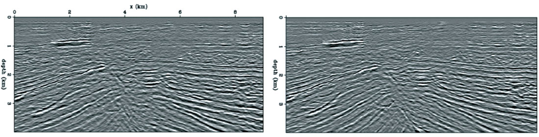
Figure 19 shows segments of seismic sections obtained by Woodward et al., with prestack depth migration using velocities obtained by conventional velocity analysis (Figure 19(a)) and by using a velocity field refined by reflection tomography (Figure 19(b)). Significant improvements in the seismic image are obtained by updating the velocity field using reflection tomographic. As shown in figure 20, Sayers et al., 2002 demonstrate the difference in pore pressure prediction by using the tomographic approach explained above. The tomographically refined velocity model yields a pore pressure spatial distribution that is easy to understand and comprehend.

Zhou at al 2004 have described a tomographic velocity analysis method in which interval velocities and anisotropy parameters are first estimated and then incorporated into the ray tracing to flatten events in the common image gathers. For anisotropic media, this process helps image subsurface structures accurately.
For areas that have lateral velocity variations and are structurally complex, tomographic inversion gives more accurate velocity models and also justifies the extra effort and cost.
6. Residual velocity analysis
One of the serious problems in doing AVO analysis is obtaining precise stacking velocity measurements for its proper application. Velocity errors that have little to no affect on conventional stacking can cause significant AVO variation several times larger than those predicted by theory (Spratt, 1987). Shuey’s formulation for AVO yields an intercept and a gradient stack. While the intercept represents the zero offset reflection coefficients, the gradient is a measure of the offset dependent reflectivity. Swan, 2001 studied the effect of residual velocity on the gradient and developed a methodology to minimize the errors by utilizing a new AVO product indicator which he called the Residual Velocity Indicator (RVI). This indicator equals the product of AVO zero offset stack and the phase quadrature of the gradient. The sign of the correlation indicates whether the NMO velocity is too high or too low. The optimal NMO velocity is the one which minimizes this RVI correlation. Residual velocity analysis produces a null point at every sample point, which facilitates the generation of a velocity value at every data sample. Thus a high resolution velocity field is generated. So, while traditional stacking velocities are generally picked with semblances, optimum velocities for AVO are picked using RVI, which is more sensitive to velocity variations than a standard semblance estimate. The residual velocity method, which was popularized by ARCO with the AVEL algorithm, also allows accurate prediction of velocities in the presence of type II polarity-reversing AVO events which cause problems for traditional semblance analysis. Spatial and temporal averaging forms part of the process to obtain a smooth and a continuous residual velocity estimate.
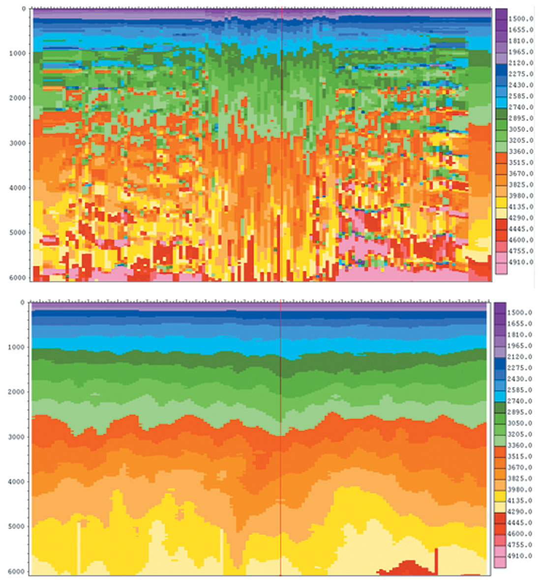
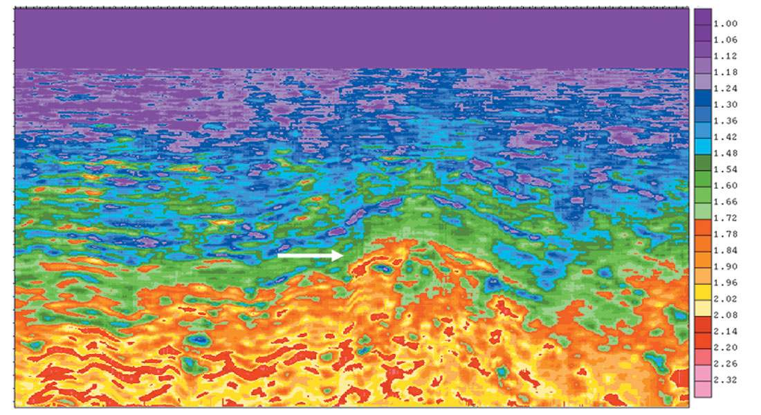
Figure 21 (a) shows an example of traditional dense velocity analysis and the smoothed equivalent velocity field used for migration (figure 21b) from Huffman et al., (2003). This section shows virtually no details of the underlying velocity field. Figure 22 shows the same section after application of residual velocity analysis. Note the details in the velocity field that follow the reflectors, including a type II AVO gas reservoir (white arrow) that displays a low velocity in a section with little stacked amplitude. This aspect of the residual velocity technique makes it particularly valuable as a data conditioning tool for geopressure, AVO and inversion studies.
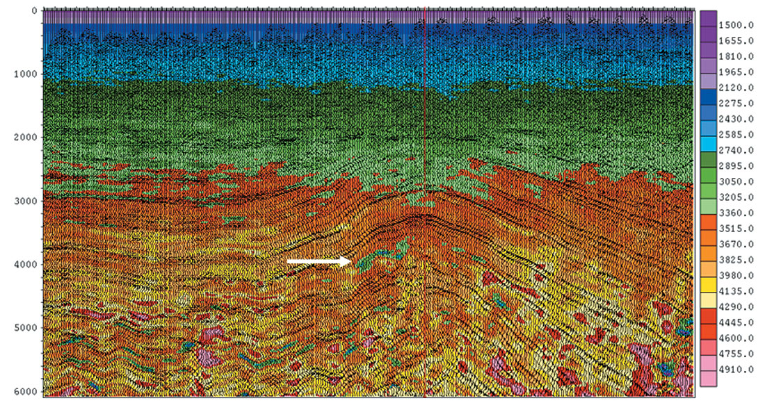
Figure 23 shows the result of transforming the velocities in figure 22 into pore pressure gradient in equivalent density units. The resulting section demonstrates the level of detail that can be derived in pressure prediction using residual velocities. The figure also demonstrates a pitfall of pressure prediction where hydrocarbons are present. The gas reservoir identified in the velocity display in figure 22 shows an anomalously high pore pressure in figure 23 which is actually caused by the gas effect in the pay zone, and is not a pressure-related effect. It is important to note that hydrocarbon effects and non-clastic rocks such as carbonates and volcanic rocks violate the calibration assumptions for pressure prediction, and thus will give erroneous pressure values. The residual velocities can in some cases allow the user to isolate these zones so that they don’t negatively impact the overall prediction process.
The computation of residual velocities uses a number of assumptions, an important one being that the velocity is assumed as constant and that AVO behaviour is consistent in the RVI window. Short offset for moveout and AVO analysis is another assumption. Ratcliff and Roberts (2003) showed that these and other assumptions are often invalid in real data and this adds noise and instability to the iteration process. By monitoring the convergence criteria it is possible to reduce or avoid these instabilities.
Ratcliff and Roberts extended Swan’s method in that once RVI estimates are computed, they are used to update the velocity field and any subsequent moveout correction. AVO analysis is repeated on the revised gathers and another residual velocity is calculated. This process is iterated until convergence occurs. This reduces the side effects mentioned above.
7. Velocities from Seismic Inversion
Seismic inversion plays an important role in seismic interpretation, reservoir characterization, time lapse seismic, pressure prediction and other geophysical applications. Usually, the term seismic inversion refers to transformation of post-stack or prestack seismic data into acoustic impedance inversion. Because acoustic impedance is a layer property, it simplifies lithologic and stratigraphic identification and may be directly converted to lithologic or reservoir properties such as pseudo velocity, porosity, fluid fill and net pay. In such cases, inversion allows direct interpretation of three-dimensional geobodies. For geopressure prediction, inversion can be implemented as a means to refine the velocity field beyond the resolution of residual velocity analysis, and also as a means to separate unwanted data from the pressure calculations.
The preferred methodology for implementing inversion for geopressure prediction is to start with a 3D residual velocity field (e.g. figure 21b) that can be used as a low-frequency velocity field to seed the inversion. The inversion is then used to refine the velocity field using the reflectivity information contained in the stacked data or gathers to provide the high-frequency velocity field.
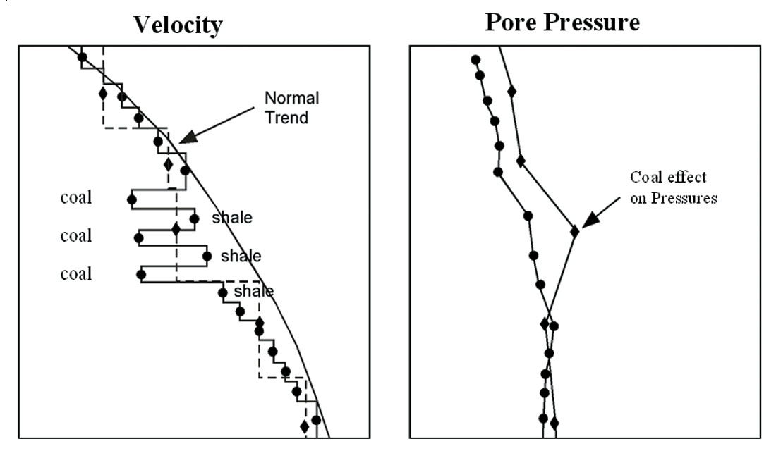
As noted earlier, it is often observed during pressure prediction that certain layers violate the rules of the prediction process. Such layers, which include non-clastic rocks like carbonates and volcanics, coals, and marls, and reservoirs affected by hydrocarbon effects, essentially violate the premise of the pressure calibration because they have very different compaction behaviors from clean shales that are used to build a typical primary compaction curve. These layers are usually embedded in the seismic velocity field so that they can’t be easily separated from the shales and sands that do follow the rules of the game. Let’s consider a case where a shale section has multiple coal seams embedded in it (figure 24). In this situation, the seismic velocity field is too coarsely sampled in time to see the coals as separate layers as shown in the dashed velocity profile. When this velocity profile is used to predict pore pressure, the low-velocity coals cause an anomalously high pressure estimate that is false. The application of inversion in such an example (the solid velocity curve) allows the coals to be separated out from the shales by manually picking the coals for removal, or by using horizons to exclude the coals from the pressure calculation. In this case, the pressure prediction follows the shales properly and the prediction is correct. This concept can be applied to any exotic velocity effect from non-clastic rocks or for hydrocarbon effects in reservoirs.
Poststack inversion
Since the inversion process transforms seismic amplitudes directly into impedance values, special attention needs to be paid to their preservation. This insures that the observed amplitude variations are related to geological effects. Thus, the seismic data should be free of multiples, acquisition imprint, have high S/N ratio, zero-offset migrated and without any numerical artifacts. Due to the band limited nature of the seismic data, the lack of low frequencies will prevent the transformed impedance traces from having the basic impedance or velocity structure (low frequency trend) crucial to making a geologic interpretation. Also, the weak high frequency signal components or their absence thereof from the seismic data will find the impedance sections wanting in terms of resolution of thin layers.
The low frequency trend of acoustic impedance is usually derived from well logs or stacking velocities and used as a priori information during the inversion process. This helps enhance the lateral consistency of the impedance data so produced. The weak high frequency signal components indicate notches or roll-offs on the higher end of amplitude spectra of seismic traces. Processing steps that tend to broaden the spectral band are usually adopted so that the data that is input to inversion has an enhanced effective frequency band-width.
Several different techniques/methodologies are commonly used to perform acoustic impedance inversion. The prominent ones are recursive, blocky, sparse-spike, stratigraphic and geostatistical inversion (Chopra and Kuhn, 2000).
All the above model based inversion methods belongs to a category called local optimization methods. A common characteristic is that they iteratively adjust the subsurface model in such a way that the misfit function (between synthetic and actual data) decreases monotonically. In the case of good well control, the starting model is good and so the local optimization methods produce satisfactory results. For sparse well control or where the correlation between seismic events and nearby well control is made difficult by fault zones, thinning of beds, local disappearance of impedance contrast or the presence of noise, these methods do not work satisfactorily. In such cases global optimization methods, e.g. simulated annealing, needs to be used. Global optimization methods employ statistical techniques and give reasonably accurate results.
Thus whatever inversion approach is adopted i.e. constrained, stratigraphic, the acoustic impedance volumes so generated have significant advantages. These include increased frequency bandwidth, enhanced resolution and reliability of amplitude interpretation through detuning of seismic data and obtaining a layer property that affords convenience in understanding and interpretation.
Prestack inversion
While poststack seismic inversion is being used routinely these days, the results can be viewed with suspicion due to the inherent problem of uniqueness in terms of lithology and fluid discrimination. Variations in acoustic impedance could result from a combination of many factors like lithology, porosity, fluid content and saturation or pore pressure. Prestack inversion helps in reducing this ambiguity, as it can generate not only compressional but shear information for the rocks under consideration. For example, for a gas sand a lowering of compressional velocity and a slight increase in shear velocity is encountered, as compared with a brine-saturated sandstone. Prestack inversion proves useful in such cases.
The commonly used prestack inversion methods, aimed at detecting lithology and fluid content, derive the AVO intercept and AVO gradient (Shuey, 1985) or normal incident reflectivity and Poisson reflectivity (Verm and Hilterman, 1995) or P- and S- reflectivities (Fatti et al., 1994). Fatti’s approach makes no assumption about the Vp/Vs and density and is valid for incident angles up to 50 degrees. The AVO derived reflectivities are usually inverted individually to determine rock properties for the respective rock layers. The accuracy and resolution of rock property estimates depend to a large extent on the inversion method utilized.
A joint or simultaneous inversion flow may simultaneously transform the P- and S- reflectivity data (Ma, 2001) into acoustic and shear impedances or it may simultaneously invert for rock properties starting from prestack P-wave offset seismic gathers (Ma, 2002). Simultaneous inversion methodology extracts an enhanced dynamic range of data from offset seismic stacks, resulting in an improved response for reservoir characterization over traditional post stack or AVO analysis (Fowler et al., 2002).
Prestack inversion for rock properties has been addressed lately using global optimization algorithms (Sen and Stoffa, 1991, Mallick, 1995, Ma, 2001, Ma, 2002). In these model-driven inversion methods, synthetic data are generated using an initial subsurface model and compared to real seismic data; the model is modified and synthetic data are updated and compared to the real data again. If after a number of iterations no further improvement is achieved, the updated model is the inversion result. Some constraints can be incorporated to reduce the non-uniqueness of the output. These methods utilize a Monte Carlo random approach and effectively find a global minimum without making assumptions about the shape of the objective function and are independent of the starting models.
Mallick (1999) presented a prestack inversion method using a genetic algorithm to find the P- and S- velocity models by minimizing the misfit between observed angle gathers and their synthetic computations. On the Woodbine gas sand dataset from East Texas, he showed a comparison of prestack inversion with post stack recursive inversion, and demonstrated that prestack inversion showed detailed stratigraphic features of the subsurface not seen on the post stack inversion. This method is computer intensive but the superior quality of the results justifies the need for such an inversion.
Example
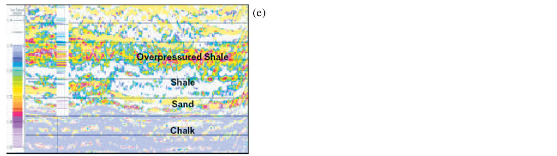
The sonic and velocity log-derived porosity trends from offshore Ireland suggest overpressures within Tertiary shale sequences. Analysis of seismic velocities for this area suggest normal shale compaction for most of the Tertiary overburden, except in certain lithologies where overcompaction is seen. The stacking velocities picked on a coarse grid and were not horizon consistent, so look blocky as shown in Figure 25(a). If there are lateral velocity variations, as seen in this case, this approach is not suitable for pore pressure analysis. In order to obtain accurate and high resolution seismically derived velocities, several iterations of the prestack depth migration using tomography was attempted. The grid based tomography provides an optimum seismic image as well as the velocity section shown in Fig. 25(b) corresponding to Fig. 25(a). Next prestack seismic inversion was attempted using Ma’s (2001) approach to be able to predict different lithologies in terms of P- and S- impedances and the two equivalent sections are shown in Fig. 25(c) and (d).
Terzaghi’s effective principle was then used to transform the seismic inversion derived impedance to pore pressure. The equivalent section shown in Fig. 25 (e) shows overpressured shales as anticipated in this area. Such information provides assurance for development well locations.
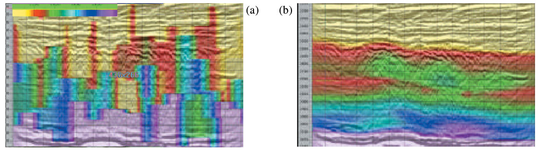
Figure 25(b). Interval velocity section obtained using reflection tomography approach.
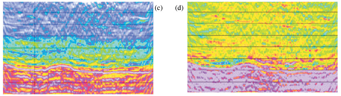
Figure 25(d). S-impedance section obtained with prestack joint inversion.
Discrepancies Between Wellbore and Seismic Velocities
One of the challenges in performing geopressure prediction with seismic velocities is that the seismic and wellbore velocities often do not calibrate properly against each other. When this occurs, an obvious question arises regarding which data type provides the best base calibration for geopressure. While this topic is beyond the general scope of this review, a few words should be said about this important topic. The issue not only affects the calibration for pressure, but also has an impact on the time-depth conversion that is required to equate the seismic velocities in time to pressure profiles in depth that are used for drilling wells.
While sonic velocities provide the highest resolution of the available velocity data, the sonic velocities often don’t provide the best calibration for seismic-based prediction because of differences in the frequency of measurement compared to seismic data and due to invasion and other deleterious wellbore effects. In many cases, the sonic and seismic can’t be reconciled, which then requires that the seismic be used to calibrate directly to avoid a mis-calibration when the jump is made from the sonic log to seismic data. In contrast, VSP and check shot data are measured at the same frequency as the seismic data, but provide a higher resolution velocity field that can be calibrated to the sonic in depth as well. Consider the example shown in figure 26.

In this case, a seismic velocity function at a well location was compared to the check shot survey and the sonic log from the well. On inspection, the interval from 1900 to 2300 meters revealed a discrepancy between the sonic and the seismic velocities. Further inspection revealed that the check shot data agreed with the sonic log from 1900 to 2150 meters, but from 2150 to 2300 meters, the check shot agreed with the seismic velocity function. Note the impact that this discrepancy has on the pressure prediction. Such differences are commonplace, so addressing them is something that every pressure analyst will face. In this particular case, the discrepancy was easily explained. The upper zone from 1900 to 2150 meters was a thick complex gas reservoir that affected the sonic log and the check shot survey but was not detected by the seismic velocities. In contrast, the zone from 2150 to 2300 meters was a zone that was affected by severe invasion of the formation by drilling mud after the mud weight was raised to manage the gas kick in the zone above. This mud invasion, coupled with dispersion effects in the sonic log, conspired to make the sonic read too fast. In this

Acknowledgements
We appreciate the constructive comments received by an anonymous reviewer that helped us improve the contents of this paper. We thank Colin Sayers and Graeme Gordon for allowing us to use figures 19, 20 and 25 and also gratefully acknowledge the permission accorded to us by SEG, EAGE and CSEG, for use of some of the other examples cited in the paper. We would also like to thank Arcis Corporation, Calgary and Fusion Petroleum Technologies, Houston for permission to publish this paper.


Join the Conversation
Interested in starting, or contributing to a conversation about an article or issue of the RECORDER? Join our CSEG LinkedIn Group.
Share This Article