Hydraulic fracturing normally creates only small magnitude events: the microseismicity that is often used to image the fracture growth. These weak microseismic events have magnitudes less than zero, and are often challenging to even detect on surface let alone be felt. However, concern is rising associated with hazards associated with larger magnitude events that might be felt on surface. A few cases of larger earthquakes have recently been reported. In Oklahoma, an earthquake with a magnitude of Md=2.8 (duration magnitude estimated from the seismogram coda) may have been related to hydraulic fracturing (Holland, 2011). In the UK during April and May of 2011, hydraulic fracturing near Preese Hall resulted in an event with magnitude ML=2.3 (local magnitude scale) and later another ML=1.5 (de Pater and Baisch, 2011). Between 2009 and 2011, 38 earthquakes including a ML=3.8 resulted from hydraulic fracturing in the Horn River Basin shale gas reservoir in north-east British Columbia, Canada (BCOGC, 2012). No physical damage or injury was reported for any of these cases, although public attention in the UK case did result in a temporary hydraulic fracturing moratorium. The UK moratorium was eventually lifted after detailed studies and recommendations for seismic monitoring with operational protocols tied into a ‘traffic light’ system, using magnitude levels of any seismicity associated with future developments.
Induced seismicity is a well-known phenomenon and can be caused by mining, reservoir or dam impoundment, and injection (McGarr et al., 2002). For example, fluid injection in Denver, Colorado in the 1960’s resulted in felt earthquakes (Healy et al., 1968), which lead to the Rangely experiment in the early 1970’s showing that seismicity could be induced and controlled through injection (Raleigh et al., 1976). Various recent examples of induced seismicity have been attributed to larger fluid injection volumes for stimulation of geothermal reservoirs (e.g. Basel, Switzerland, for example see Shapiro et al., 2010) and waste water injection (Dallas-Fort Worth, Texas; Guy, Arkansas; Prague, Oklahoma; Raton Basin, Colorado; and Youngstown, Ohio: for a comprehensive review of various examples included here see National Research Council report, 2012). In a number of the waste-water disposal-induced seismicity cases, produced water from hydraulic stimulated wells was being re-injected. However, the injection volumes are typically significantly larger than even the largest hydraulic fracture stimulations in unconventional reservoirs.
Hydraulic fracture stimulation associated with creation of new fractures and interaction with pre-existing fractures results in small magnitude ‘induced microseismicity’. The microseismicity is classified as induced in that it would not otherwise have occurred if not for the hydraulic fracture. The magnitudes vary depending of the site conditions and hydraulic energy (Maxwell et al., 2008), but at some instances are too small to be recorded even using sensitive downhole recorders at close proximity. In other reservoirs, particularly those at a high stress level or when faults are activated, the magnitudes can increase. Magnitudes also increase when the hydraulic fracture grows into a fault, where the increased pressures from the fracturing can induced the fault to move. Microseismic monitoring has been performed in many reservoirs to image hydraulic fracturing. In most reservoirs, the magnitudes are found to be below magnitude -1, but in some cases the events can reach 0 or slightly higher. Indeed, of the hundreds of thousand hydraulic fractures that have been performed, only the three cases mentioned above (i.e., OK, UK and BC) have induced seismicity been reported. Therefore, the cases of the felt seismicity resulting from hydraulic fracturing can be considered both rare and anomalous.
A large fault plane is required to create the movement required to generate larger magnitude events. The fault is also likely carrying enough tectonic stress for sufficient fault movement to result in seismicity. Thus, the fault movement causes unintentional ‘triggered seismicity’ resulting from the release of tectonic stress as opposed to the intentional ‘induced microseismicity’ that wouldn’t have occurred without the fracturing itself. McGarr et al. (2002) describes induced seismicity as scenarios where there is a significant change relative to the ambient stress versus triggered where only a relatively small change causes the seismicity. Nevertheless, the terms triggered and induced seismicity often tend to be used interchangeably. Since small pressure and stress changes can occur for some distance around the hydraulic, triggered fault activation could potentially occur remotely from the hydraulic fracture.
In order to mitigate the risk associated with induced seismicity, a number of different operational protocols have recently been proposed. Each of these protocols includes characterization of the potential of induced seismicity, assessment of the impact of injection and seismic monitoring. These are typically an iterative workflow, since seismic monitoring can refine or possibly identify fault structures and also help constrain the predictions. Each protocol utilizes a monitoring system and the observed seismicity to make operation decisions about when it is safe to proceed, using so called ‘traffic light systems’. The following discusses particular aspects of these protocols and reviews various aspects of anomalous seismicity associated with hydraulic fracturing. In particular, a tutorial is provided about estimate source magnitudes, including possible processing pitfalls. Empirical energy and injection volume balances are also discussed as potential methods to estimate the largest possible magnitudes and monitoring techniques to provide context for interpreting the seismicity levels.
Operational Protocols
Three distinct operational protocols have been proposed: from the US Department of Energy (DOE) for geothermal operations, hydraulic fracturing from UK Department of Energy and Climate Change (DECC) and Canadian Association of Petroleum Producers (CAPP).
DOE Geothermal Injection Induced Seismicity Protocol
The US Department of Energy developed a protocol specifically for geothermal projects (Majer et al., 2012). However, the protocol can also be used for other injection programs. The following are the proposed steps:
- Perform preliminary screening evaluation
- Implement an outreach and communication
- Review and select criteria for ground vibration and noise
- Establish local seismic monitoring
- Quantify the hazard from natural and induced seismic events
- Characterize the risk of induced seismic event
- Develop risk-based mitigation plan
The proposed risk-based mitigation plan describes using ground motion in a traffic light system.
UK DECC Hydraulic Fracturing Induced Seismicity Protocol
After the magnitude 2.3 Presse Hall event in April 2011, a temporary moratorium was imposed through the UK while the occurrence was studied. Eventually, the moratorium was lifted with a highly publicized protocol relying on a magnitude based traffic light system (Green et al., 2012):
- Pre-fracture assessment of seismic risk and faults
- Submission of a pre-fracture plan for addressing seismic risk
- Seismic monitoring (before, during and after)
- Magnitude based traffic light system, to modify (amber) and potentially halt (red) operations at mag 0.5
CAPP Hydraulic Fracturing Induced Seismicity Protocol
Following the identification of hydraulic fracturing induced seismicity in the Horn River Basin in NE BC, the Canadian Association of Petroleum Producers (CAPP, 2012) also released a suggested protocol which is summarized below:
- Assess faults, lineations, background seismicity and other possible cases of induced seismicity in the area
- Develop initial operational protocol including tracking local seismicity and any felt events, and microseismic monitoring if available
- React and elevate monitoring if something is observed
Although effectively including a magnitude based traffic light system tied into detection, the national NRCAN monitoring array is also suggested as a backbone of the proposed monitoring supplemented with observations of seismicity being felt on surface.
Each of the protocols above follows the same basic workflow of characterization, assessment, monitoring and reaction to mitigate hazard. However there are many specific aspects to this overall workflow, which will be further reviewed in the subsequent discussions.
Criteria for Identifying Induced Events
In some cases it can difficult to establish cause and affect relationships between injection and seismicity in order to determine that the seismicity was induced by the injection activity. Davis and Frohlich (1993) proposed seven questions which are often used as an objective test:
- Are these events the first known earthquakes of this character in the region?
- Is there a clear (temporal) correlation between injection and seismicity?
- Are epicenters near wells (within 5 km)?
- Do some earthquakes occur at or near injection depths?
- If not (similar depth) are the known geologic structures that may channel flow to sites of earthquakes?
- Are changes in fluid pressure at well bottoms sufficient to encourage seismicity?
- Are changes in fluid pressure at hypocentral locations sufficient to encourage seismicity?
It can be challenging to clearly and unambiguously identify a specific seismic event in question as either induced or natural. These questions are meant to provide ‘rational criteria’ to establish if an event is induced, as is designed for a generic injection scenario. However, in the specific case of hydraulic fracturing question 6 is always yes since treatments are at by definition at fracturing pressure.
Establishing the background seismicity level is an important aspect. A baseline recording of significant time is critical to establish accurate background seismicity levels. Inevitably monitoring arrays are installed as questions of induced seismicity occur effectively increasing the sensitivity after the fact and complicating the comparable baseline monitoring. Furthermore, natural seismicity is often a very slow process, requiring a long database to statistically categorize levels. Often historical seismicity information is lacking, and regional seismic networks may not have the sensitivity to detect small magnitude events. Therefore it can be difficult to confidentially establish if suspect seismicity is anomalous to the region.
In some cases, the initial local seismic monitoring system may also not be sufficiently dense to allow confident event locations. With a relatively large hypocentral error, causal relations can be more difficult to establish. Uncertainty in location can also lead to ambiguity in the hydraulic fracturing operation that triggered the seismicity, in scenarios where multiple companies are operating relatively close together. In some recent cases, suspected induced seismicity may also occur at distance from the injection and potentially deeper than the injection point.
Establishing a temporal correlation can also be a challenge in certain cases, especially for long term injection when suspected seismicity may occur some time after the injection first begins. Temporal correlation needs to be carefully considered, since post injection induced seismicity has occurred after the injection has stopped (for example, Basel Switzerland). Post-injection induced seismicity can be a challenge to identify, especially if seismicity is absent or low level during the injection.
The above criteria obviously rely on seismic monitoring: clearly the more sensitive and accurate the better.
Measuring Seismic Source Strength
Characterizing seismic source strength is obviously an important topic, particularly since many induced seismicity mitigation practices rely on a ‘traffic light’ monitoring systems. These traffic light systems define operation protocols tied in to observed magnitude thresholds.
Seismic sources are typically characterized using either a measure of the causal source strength or, alternatively, the resulting intensity of ground shaking. For example, the Modified Mercalli Intensity Scale uses 12 levels to quantify the human perception and damage associated with an earthquake, reducing in intensity with distance from the source. Earthquake ‘shake maps’ can also be used to estimate instrumentally derived intensities using observed ground motions in areas with sufficient density of seismometers.
| Magnitude | Typical Modified Mercalli Intensity | Effects |
|---|---|---|
| Table 1. Modified Mercalli Intensity and approximate magnitude for near-by events (after USGS). | ||
| Below 3 | I | Instrumental, not felt |
| 3 to 3.9 | II to III | Perceptible, vibration similar to a truck passing |
| 4 to 4.9 | IV to V | Generally felt, dishes rattle |
| 5 to 5.9 | VI to VII | Slight to moderate damage |
| 6 to 6.9 | VII to IX | Moderate to heavy damage |
| Above 7 | X or higher | Significant damage |
Magnitude estimates are the other common source characterization, providing a measure of the strength of the source itself. The well known Richter magnitude is one such measurement scale belonging to a general class of local magnitude scales (ML) computed from an empirical relation between the observed instrumental seismic amplitude and source-receiver distance:

where A is the observed amplitude and R is the source-sensor distance and B and C are constants depending on the calibrated scale used. Various magnitude scales have been empirically calibrated for consistency over some magnitude range with the original Richter magnitude. In terms of microseismicity and activity with negative magnitudes, it is interesting to note that the Richter scale was originally proposed to avoid computed magnitudes below zero. However with modern recording instruments significantly smaller amplitudes can now be recorded than in the 1930’s and negative magnitudes are routinely recorded during microseismic surveys.
A more robust magnitude scale is the moment magnitude (MW) based on the scalar seismic moment (M0), which has a physical definition for a fault displacement:

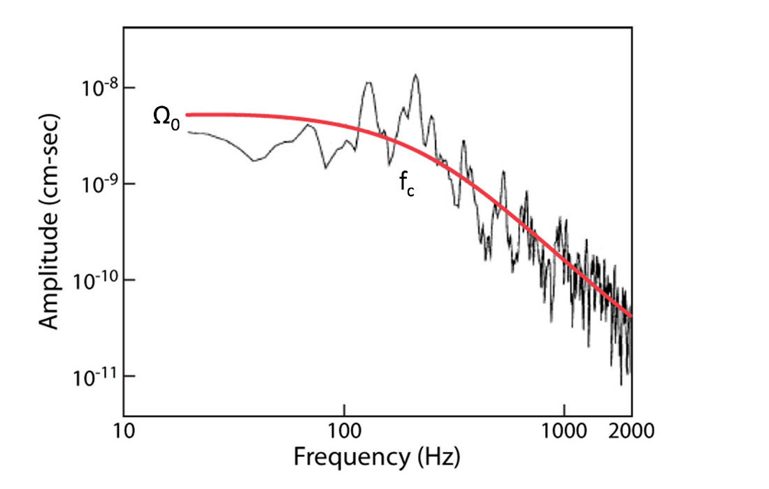
where µ is the shear modulus, A is area of slip and d is the displacement of slip. Seismic moment can be estimated from the frequency content of the recorded seismic waves. Figure 1 shows a spectral plot of a seismic signal along with a source model fit of the form (e.g. Abercrombie, 1995):

where Ω0 is a low frequency plateau value, fc is known as the corner frequency and Q is the seismic quality factor accounting for signal attenuation. The low frequency plateau is then used to estimate the seismic moment:

where ρ is density, c is the velocity of the phase being modeled, R is distance from source to receiver, and Fc is the radiation pattern. If the focal mechanism is unknown, an average radiation pattern coefficient of Fα = 0.52 and Fβ = 0.63 (Boore and Boatwright, 1984). The seismic moment can be expressed (Hanks and Kanamori, 1979) as the moment magnitude:

which is a magnitude scale valid across scales from larger tectonic to weak microseismicity.
Accuracy of Magnitude Estimates
Moment magnitudes are the preferred measurement scale for reporting induced seismicity and microseismicity associated with hydraulic fracturing (e.g. Maxwell et al., 2008). Recorded magnitudes are a critical component of quality control of microseismic data sets, and can be used to establish the relative recording sensitivity, identify and correct for monitoring biases, identify fault activation and help define the effectiveness of the stimulated reservoir volume. Obviously microseismic magnitudes are also important for investigating potential anomalous induced seismicity, both in terms of typical magnitude levels in an area including both induced and background tectonic activity and monitoring for magnitude traffic light systems. Clearly, traffic light systems and associated protocol magnitude thresholds require a clear definition of which magnitude scale is to be used. However, caution is needed to avoid potential errors in the estimated magnitudes.
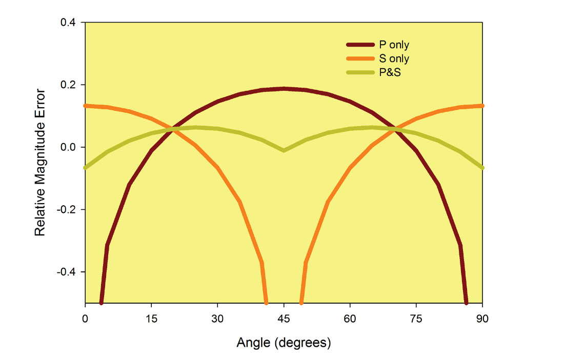
Errors can occur with the conversion of measured seismic amplitudes from recorded signals to true ground motion parameters. However, due diligence and proper calibration can easily overcome this factor. Often microseismic magnitudes are estimated without knowledge of the seismic radiation pattern, and average radiation patterns are used. Average radiation patterns are intended to average out over arrays sampling the radiation pattern in different directions. Since many microseismic monitoring projects are performed with single well arrays, it is important to consider potential magnitude errors associated with the average radiation patterns described above. Figure 2 shows potential errors in magnitudes for different angles of the fault plane relative to the monitoring direction to a single borehole array. As shown in the figure, significant errors occur in specific directions where the magnitude is underestimated if only one phase (i.e. only Por S-waves) is used for the magnitude estimation. However, using both phases simultaneously tends to cancel the source directivity effect of a single phase. Errors can also occur if the fracturing mode is not a shearing mechanism as assumed in Figure 2 and in the average radiation patterns, and other magnitude estimation formulation are needed.
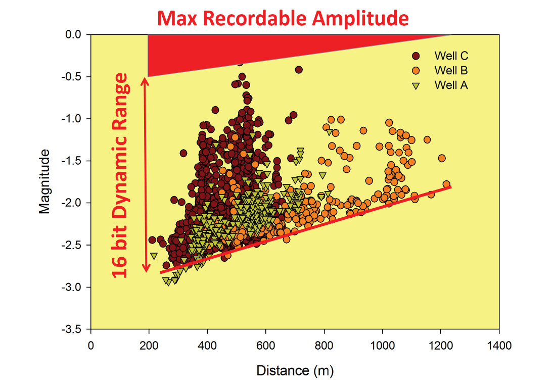
The recording system dynamic range (i.e. range of amplitudes that can be measured) is also relevant and a potential source of error. Many microseismic monitoring systems use a 24-bit acquisition system with a specific maximum amplitude that can be recorded before the seismic waveforms are clipped, as they exceed the voltage limitation. Figure 3 shows a schematic illustration of the maximum magnitude that could be recorded prior to clipping. If signal amplitudes exceed these values, the waveforms can potentially be clipped and the magnitude may be under estimated. Signal clipping is easy to identify and flagged for uncertainty in the reported magnitude. Alternatively, some acquisition systems are capable of varying the system sensitivity on a sensor-bysensor basis, in which case certain sensors in the array could use a lower sensitivity to estimate magnitudes on larger events to effectively extend the dynamic range.
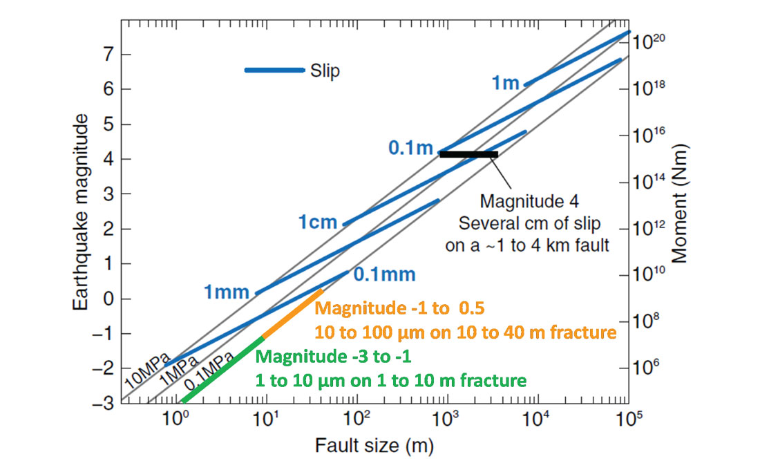
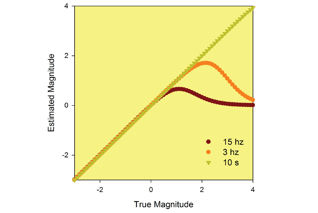
The recording system frequency bandwidth is also potentially a factor in confident magnitude estimations. Figure 4 shows an earthquake magnitude scaling diagram, showing how increasing earthquake magnitudes are associated with slip on larger faults. Estimated fault size in inversely proportional to the corner frequency (Figure 1). Therefore larger magnitude events are associated with lower seismic frequencies. Common sensors used in microseismic monitoring have relatively uniform sensitivity above about 10 Hz, and rapidly fall off in sensitivity at lower frequencies. The low frequency content of the signals can be partially compensated by correcting for the sensor response, to enable the low frequency components in the signal below 10 Hz to be used in the source characterization. However, many of the recording systems used in microseismic monitoring also have electronic bandwidth responses that can also compromise the low frequency capabilities. Low frequency limitations can be visually identified in the recording and used to flag uncertain magnitude levels. Figure 5 shows an estimate of the source size underestimation that can occur with different sensor frequency limits. With both the clipping issue discussed above and the frequency limitation, microseismic magnitudes over about magnitude zero come into question unless specifically reviewed.
Finally, magnitude estimations also require sensors to record the far-field seismic waves a distance from the source. Far field approximations for large events may not be valid for downhole arrays close to the target zone.
Therefore, there are a number of factors that can impact the ability of a microseismic monitoring system to record and accurate estimate larger magnitudes above zero. Some of these factors can be compensated for by calibrating arrays for local magnitude estimations. However care is needed before using these reported magnitudes to monitor for larger seismicity. A preferred monitoring solution for reliable estimation of larger events is to use broad-band seismometers designed to recording earthquakes. Nevertheless, there are many projects where microseismicity is reported with accurate magnitudes well below zero, and provides a confident representation of the lack of large magnitude events.
Seismic Hazard and Risk
Beyond the characterization of the seismic event source strength, the effect and potential consequences of the seismicity is even more important. Generally seismic hazard is considered to be the probably of a certain amount of ground motion (ground shaking either in terms of velocity or acceleration) occurring and the seismic risk, is the possible consequence or resulting damage (e.g., Atkinson and Martens, 2007). Hazard is normally expressed as a probability of excedance of a specific ground motion over a specific time interval (probabilistic seismic hazard analysis, PHSA). Ground motion associated with an earthquake depends on:
- Source strength and radiation pattern
- Distance
- Attenuation
- Site conditions
The seismicity recurrence rate and probabilistic distribution of these parameters defines the PSHA, which is characterized for tectonic earthquakes to define building codes.
Compared to than tectonic earthquakes, induced or triggered seismicity associated with injection tend to be somewhat more bounded in some of the ground motion controlling factors, in that the seismicity tends to be proximal to the injection site. Since most wells are relatively shallow compared to crustal tectonic faulting, this may imply closer distances and relatively higher hazard. However, a few suspected cases of waste injection wells inducing seismicity may have resulted in deeper seismicity far below the injection.
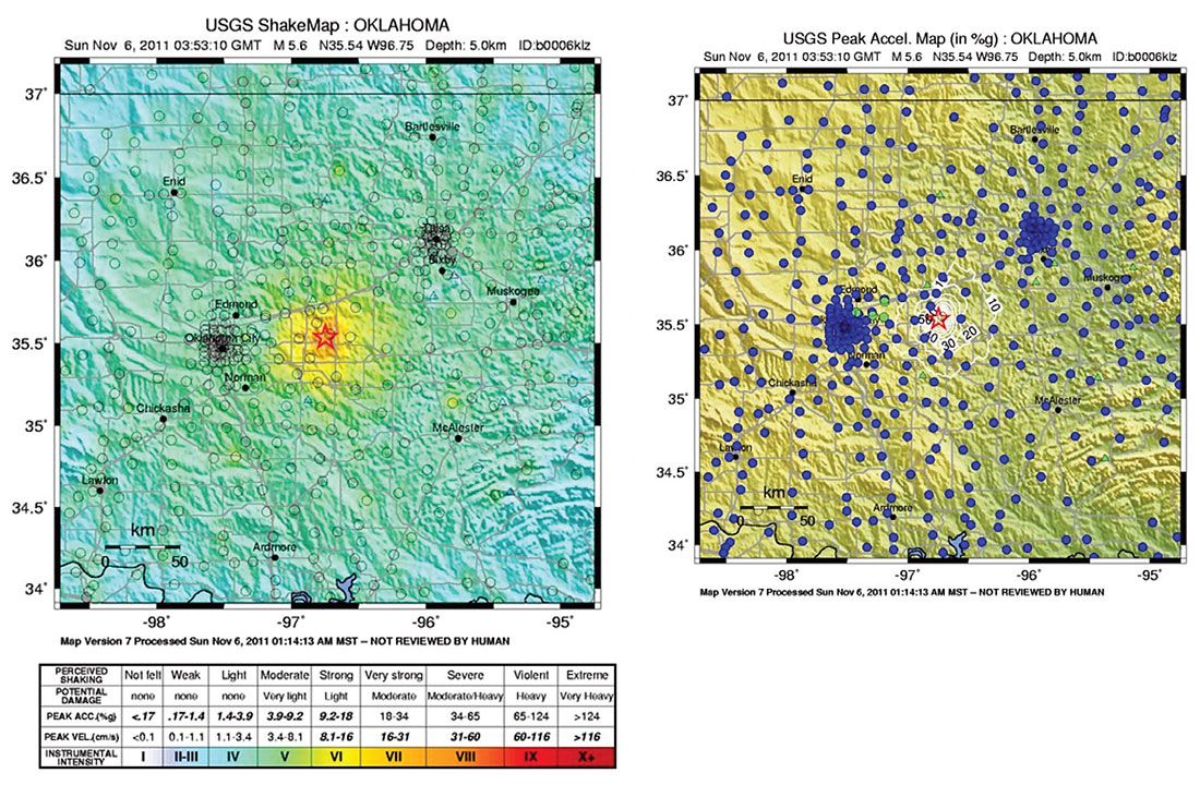
Earthquake ‘shake maps’ can also be produced from recorded peak seismic ground motion parameters to estimate instrumentally derived intensities. For example, Figure 6 shows a map of peak ground acceleration and estimated intensity for the November 6, 2011 Prague Oklahoma earthquake (magnitude 5.6) thought to be related to regional injections.
It is interesting to note that many proposed traffic light systems are based on estimated magnitude scale estimation of source strength, as opposed to estimates of peak ground motion. Ground motion obviously is the attribute directly related to hazard, and for the reasons described above there can be range of ground motion levels associated with a specific magnitude level. However, often surface station density is too low to provide a reasonable shake map for local seismic events. Therefore, magnitude provides a useful characterization for operational protocols.
Geomechanical and Geological Conditions
In order to generate a large magnitude event, a sizable fault surface is required. Normal scaling relations suggest at least a 200 m length fault for a magnitude 3. The fault also must be under significant tectonic stress and likely either seismically active with previous seismicity or have seismicity on regional faults. A larger fault is unlikely to be created in the case of induced seismicity, and the seismicity is more likely activation of pre-existing faults where the hydraulic fracture induced or potentially triggered movement. Identifying faults is important and can be achieved from seismic reflection images, and possibly confirmed with core, image logs or even possibly microseismicity. In some cases subseismic faults may exist and only become apparent when illuminated with microseismicity.
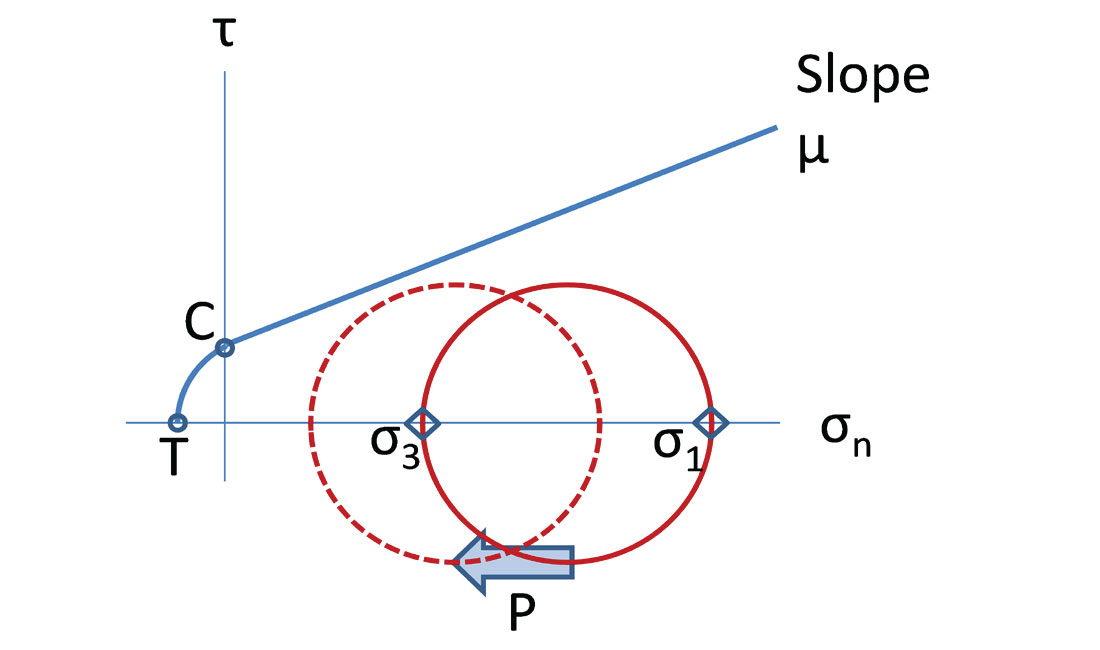
Fault movement requires sufficient tectonic stress to cause it to move. The typical mechanical model of induced seismicity is increased pore pressure associated with the injection reducing the effective normal stress on a fault allowing it slip under shear. A Mohr circle stress representation (Figure 7) illustrates the pore pressure reduction moving towards the failure or movement point as the shear driving stress overcomes friction. The closer the initial stress to the failure point (termed critically stressed if almost to the point of causing slip) the less pore pressure needed for movement. Background natural seismicity is a clear indication that tectonic stresses are already at the failure point. A hydraulic fracture itself can also locally change the stress state and cause fault slip, as the fracture dilates and pushes on surrounding rock.
Even with the existence of a large fault and shearing stress does not necessarily mean that induced seismicity will occur. A smaller patch of a large fault could slip, resulting in a smaller seismic event. Furthermore, fault slip could be ‘slow’ and the event may go unnoticed (instrumentally detected or perceived).
Prediction and Assessment
Another important aspect of both screening and making ongoing operation decisions is related to estimating the size of events that could be generated with different injection scenarios. All of the operational protocols require some form of assessment of the seismic risk, which is arguably the most challenging aspect. Of course past empirical observations can be used, potentially relying on analogues or possible nearby experiences. Nevertheless, the following three techniques can also help assess the impact and potentially provide a limit on the maximum sized event that might occur.
Geomechanical Simulation
With adequate site characterization, a computer simulation can be performed to examine pressure and stress conditions. A flow simulator can also be used to estimate the pore pressure changes during injection below fracturing pressure. During hydraulic fracturing, simulations can be used to estimate fracture deformation and associated stress changes, in addition to pressure changes both within the fracture system and due to leak-off. For both scenarios, geomechanical stress-strain simulations can be used to check for stability or fault slip, and potentially estimate the post-failure magnitudes of slip. As such the simulation of the amount of slip allows an estimate of the equivalent seismic magnitude, which can be either assumed as an equivalent single event of assuming some frequency- magnitude relationship the total (moment) magnitude. A seismic efficiency is required to estimate the radiated seismic energy portion, which is typically assumed to be several percent. McGarr (1976) reports values as low as 0.24% to 1% for mining induced seismicity. A deterministic geomechanical simulation likely requires validation of the input parameters for confident application, so typically the actual observed induced seismicity or possibly other microseismicity supplemented with pressure and strain monitoring is required. As such simulations are likely not successful in forecasting seismicity early on, although potentially useful in post-mortem analysis and examining possible operation scenarios.
Empirical Energy Balance
During a hydraulic fracture treatment, the hydraulic energy associated with the injected fluid volume can be estimated as the work done during pumping operations and can be computed as the product of injection pressure and volume. Obviously, conservation of energy must apply to the total system, so the input energy associated with the injection must equal total energy output. Energy losses associated with friction, thermal changes and fluid leak-off from the hydraulic fracture to the reservoir account for energy dissipation. The remaining portion of the hydraulic energy goes into fracture creation and dilation, with some seismically radiated in the form of microseismicity. However, the hydraulic fracture can also interact with pre-existing faults and release stored tectonic stresses, which is believed to be the mechanism of injection induced seismicity. This radiated tectonic energy depends on the properties of faults encountered, and stored tectonic energy release is in addition to the hydraulic fracture energy balance previously described. The microseismic energy (here estimated from seismic moment following Kanamori, 1978) associated with the hydraulic fracture is therefore expected to be a small portion of the total hydraulic energy, depending on the significance of the other energy factors and the incremental tectonic energy release.
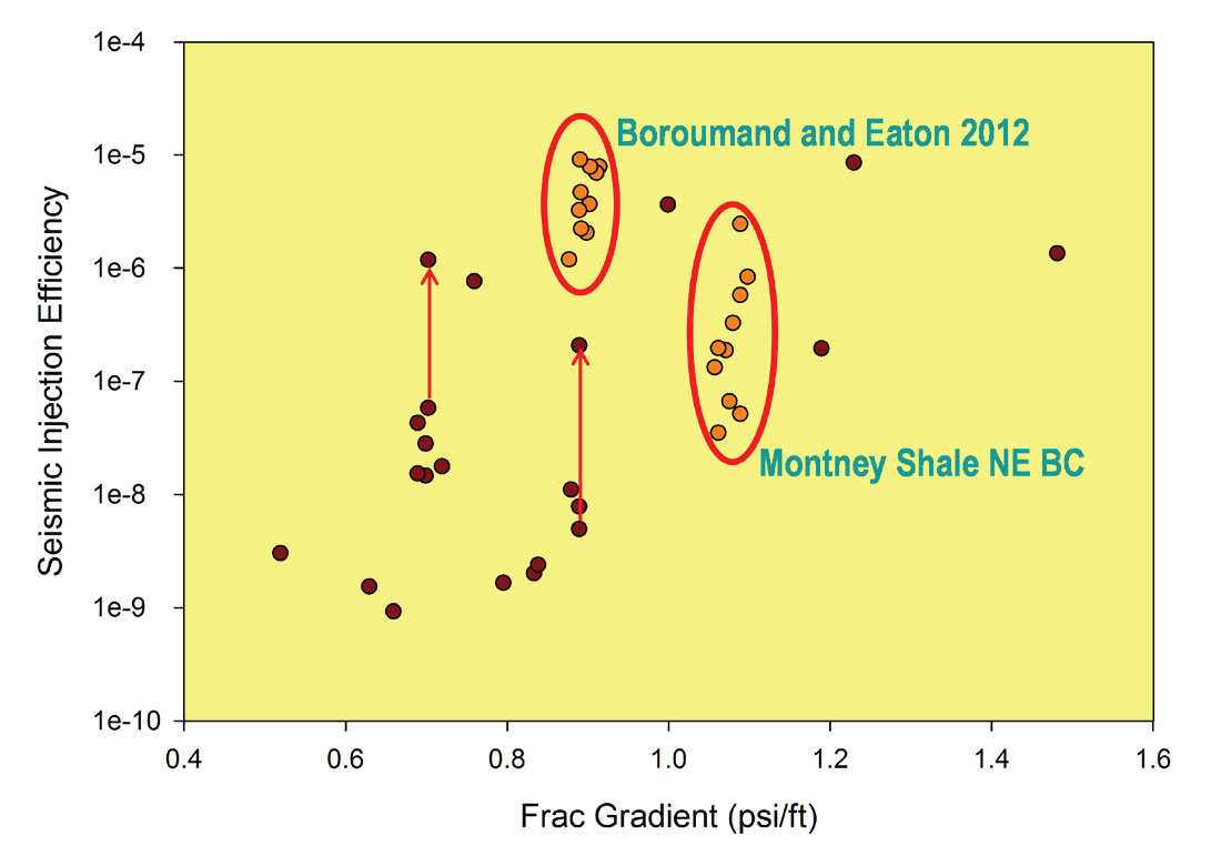
Maxwell et al., (2008) compare observed microseismic energy release from various reservoirs with the hydraulic injection energy. The comparison determined that the microseismic energy is a very small portion of the hydraulic energy with reported ratios between 1x10⁻⁹ and as large as 1x10⁻⁵. The energy ratio which was defined as the ‘seismic injection efficiency’ was found to crudely correlate with the fracture gradient (essentially a proxy for minimum stress). Examples were also reported in which the energy ratio rose because of fault activation, increasing by up to two orders of magnitude. Figure 8 shows a plot of energy ratio where fault activation examples are highlighted. Fault activation examples show the ratio prior to the fault movement along with the final point which results with a move vertically upwards in the plot to a higher ratio. The Montney Shale example also includes some stages that were interpreted to indicate fault activation, which plot at higher efficiency values. From a seismic hazard point of view, low efficiency values are preferred since seismic activity is limited to weaker microseismicity. Boroumand and Eaton (2012) computed efficiencies for Horn River Basin (HRB) in north-east BC, for a dataset with only small magnitude microseismicity below magnitude 0 (i.e., this particular dataset is not associated with induced seismicity).
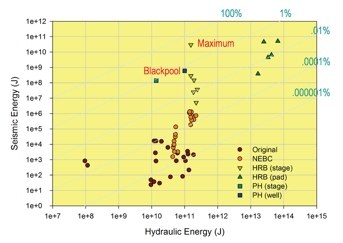
To compare with some larger magnitude events, Figure 9 shows a cross-plot of microseismic and hydraulic energy. Reference lines of efficiency are shown as percentages. Data from Figure 8, HRB and Presse Hall in the UK (PH) are included. Both of the later data sets are shown for the total seismic and hydraulic energies on a per-pad basis. For HRB the dataset involves an average of 8 wells and 17 fracturing stages per well, but PH involves just 1 well and 6 stages. Only the five HRB pads with large events are included. The two HRB pads where no earthquakes were reported would plot somewhere below these data points. For both sites, the data from the total fracture injections are plotted with the average per stage. In the case of HRB, the actual energies observed on single stages is variable, so the maximum is plotted for the one stage where the largest event (ML=3.8) occurred. Note that the range of efficiencies fall between 0.0001% to almost 50%: a variation of almost a factor of 1 million times. The increased seismic energy release is again attributed to tectonic stress release resulting from hydraulic fracturing reactivating existing faults. For all the data examined, the seismic energy release is less than the hydraulic energy consistent with observations for geothermal cases of induced seismicity (Baisch and Vörös, 2011). Therefore the energy ratio may provide a means to estimate the maximum size event, although this is speculation and not yet proven.
Empirical Volume Balance
An alternative view to energy conservation is based on the concept that the total injected volume of an incompressible fluid must be preserved. During a hydraulic fracture treatment, the injected fluid volume is precisely measured. When fracturing low-permeability shales, the injected volume must be accommodated in fracture volumes, either that of newly created hydraulic fractures or pre-existing faults and fractures. McGarr (1976) proposed a model relating total seismic moment to volume change, through either mining extraction or injection inflation. The McGarr injection model relates injected volume (V) to the total seismic moment (M0) source strength:

where k is a constant, and µ is shear modulus. The total moment can be approximated as the moment release of the strongest event, and as shown by McGarr (2013) it appears to define an upper limit on the magnitude of injection-induced seismicity from cases of anomalous seismicity during geothermal, waste injection, and hydraulic fracturing operations.
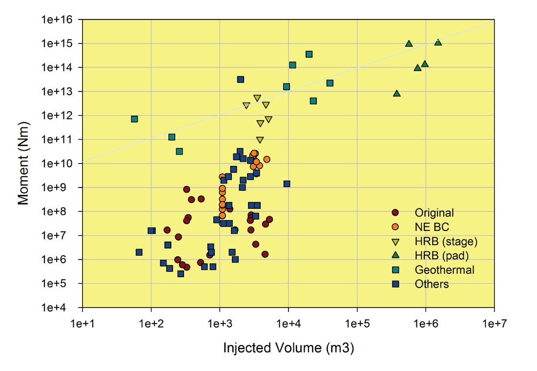
Figure 10 shows a plot of moment magnitude of the largest events versus injection volume for a series of hydraulic fractures (several published examples too numerous to cite here), both cases of large induced seismicity and a number of more typical cases with magnitudes less than zero. Also plotted are some geothermal examples (Basel, Soultz, Cooper Basin for example) of induced seismicity. Consistent with McGarr (2013), maximum magnitude associated with a typical shear modulus is shown for reference and generally follows the largest events. Data from Maxwell et al. (2008) and other published hydraulic fracture examples (too numerous to cite) are shown. These more typical cases plot well below the modulus trend with small moments below 1010 Nm and injection volumes below 10,000 m3. This is consistent with the observation that the vast majority of hydraulic fractures do not result in induced earthquakes. Nevertheless, based on the few cases of reported anomalous seismicity during hydraulic fracturing, the McGarr (1976) model appears to provide an upper limit on the maximum magnitude.
Analysis of both the energy and volume budgets during hydraulic fracturing indicates that the majority of deformation is typically aseismic. Significant energy dissipation and volumetric deformation occur without corresponding seismic radiation within the detectable microseismic bandwidth. This aseismic deformation is associated with slow fracture dilation. The exception is when hydraulic fracturing interacts with faults and tectonic stresses are released. Fault activation and the associated potential tectonic stress release result in progressively larger microseismic energy release relative to the injection energy. Based on limited observations of a few cases of stronger seismic activity, it appears that both the energy and volume budgets may provide upper limits on the size of the seismicity. From an energy perspective, the seismic energy is less than the hydraulic injection energy. Similarly, the seismic moment is less than the shear modulus times the injection volume. Of course only a small number of examples are known, so there is limited statistical sampling. Both methods of estimating an upper limit on magnitude raise an important question about the representative hydraulic energy or volume which is appropriate to use in the analysis. Progressive fracturing in a small area results in incrementally increasing total energy and injected volume. However, fracture fluid flow back and production lower the net injection energy and volume and likely also the corresponding induced seismicity. Therefore, it may not be obvious what energy or volume is pertinent.
Conclusions
Although injection can certainly induce seismicity, hydraulic fracturing using relatively small volumes, short injection times and small hydraulic energy results in only limited examples of known or suspected induced seismicity. Larger injections, such as waste water disposal and geothermal injections appear to be more associated with induced seismicity, although the number of suspect cases is still a small proportion of injection operations. Observations of suspect cases of induced seismicity suggest that the magnitudes are related to injected volumes. Nevertheless, many more examples exist for all types of injections including hydraulic fracturing where no anomalous seismicity occur and seismicity levels remain significantly less than suggested by a simple volumetric relationship. The seismic energy release is typically a very small portion of the hydraulic energy associated with a hydraulic fracture injection, with the remainder of the energy being associated with the slow, tensile hydraulic fracture deformation. In cases of induced seismicity, the seismic energy release is a more significant portion, but smaller than the hydraulic energy. Similar observations have been made for geothermal injections (Baisch and Vӧrӧs, 2011).
Both the volume and energy balances may potentially be used to estimate the maximum sized event that could be induced. Furthermore, the energy or volume ratios can be tracked with time as a means of potentially identifying scenarios leading to the occurance of induced seismicity. Energy ratios are also potentially an interesting parameter, in that if operational procedures could be modified (perhaps injection rate or duration) in such a way as to lower the energy balance and alleviate induced seismicity. While adjusting the injection in reaction to suspected induced seismicity, both the volume and energy balances can be used for context to understand the incluence of changes in the injection. Perhaps this is a way to manage controlled slow, aseismic slip, instead of suddenly releasing stored tectonic energy and avoiding anomolous seismicity.
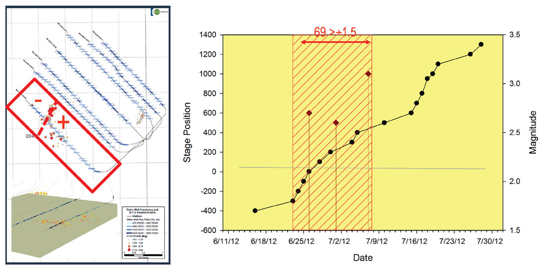
Alternatively, if faults become apparent during the course of a hydraulic fracturing, planned stages could be skipped over a portion of the well near the fault to avoid induced seismicity. For example, Figure 11 shows an example from the BCOGC report. In this case a number of seismic events over magnitude 1.5 occurred, including 3 events over magnitude 2.5. However, the elevated seismicity was localized on what was subsequently interpreted to be a fault crossing the well and began and ended with stages a certain distance on either side of the fault. With the benefit of hindsight, perhaps skipping the stages around the fault may have avoided the induced seismicity. Monitoring the energy and volume balance (i.e. ratio of seismic to hydraulic energies and ratio of cumulative moment to injected volumes) also provides an analysis method that might be useful to monitor for localized, anomalous seismic activity.
Reliable assessment of seismic hazard prior to injection remains a challenge. A critical technology for mitigation is therefore seismic monitoring: for both background monitoring and ongoing fracture monitoring. In terms of background monitoring, regional seismic arrays provide important information about regional natural seismicity and activity rates. Microseismic monitoring datasets can provide useful characterization of the magnitudes generated during fracturing in a specific area. The cases of reported induced seismicity from hydraulic fracturing occur in isolated regions, so that local hydraulic fracture microseismic data is a useful and important component.


Join the Conversation
Interested in starting, or contributing to a conversation about an article or issue of the RECORDER? Join our CSEG LinkedIn Group.
Share This Article