Uncertainty in AVO – How can we measure it?

Overview

AVO analysis has become a basic and accepted tool for both exploration and production. In this regard, it has come a long way from the early days when acceptance of the method oscillated wildly between excessive expectations and total rejection. Probably the biggest change that has come about is that geophysicists now realize that AVO is just one tool in the tool-box, providing a small but important addition to our knowledge of the prospect or reservoir. Predictions from AVO, as with all geophysical predictions, are really probability statements. When we see an AVO anomaly, we shouldn’t say “AVO shows there is gas here.” We should say: “AVO (and other factors) say there is probably gas here.” In fact, it would be very nice if we could attach a believable numerical value to that probability. This paper describes a step in that direction.

Traditional AVO Analysis

The starting point of our analysis is what we can call “Traditional” AVO analysis. Of course, there are so many approaches to AVO these days that this is a little hard to pin down. But a good starting point is shown in Figure 1.

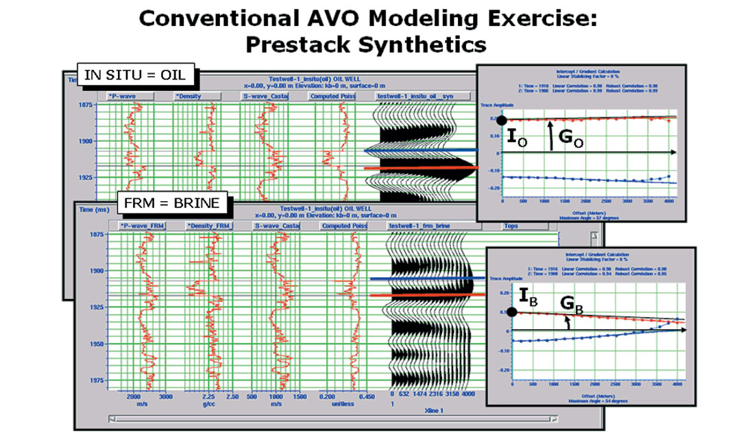
Figure 1 shows two synthetics which have been calculated from the same basic well log data. The first case, shown at the top of the figure, is the in situ oil case. The graph to the right of the synthetic shows that we can expect a small increase in amplitude with offset at both the top and the base of the target zone. The Intercept, I_O, and Gradient, G_O, are measures of the response for this case. To create the second case, shown at the bottom of the figure, fluid substitution has been used to replace the oil with brine. The change in the synthetic is reflected in the new values of Intercept, I_B, and Gradient, G_B. Theoretically, we can use this information to compare with intercept and gradient values from our real data prospect and see which category they fall into, brine or hydrocarbon. In fact, this is the basis of the currently popular cross plot method (Ross, 2000), in which we cross plot the gradient against the intercept, and identify anomalous regions on the cross plot.

But there are two immediate limitations to this procedure. The first is that we have only two modeled values which depend on a very special set of well log conditions, and there is no reason to expect the real data case to reflect exactly those conditions. The second is that we would like a numerical measure of how closely the real data values conform to any one particular model condition.

Stochastic Modeling

The solution to the first limitation is to create a large number of models, which reflect the variety of possible conditions we expect to encounter. This process, called Monte Carlo Simulation, is illustrated in Figure 2.

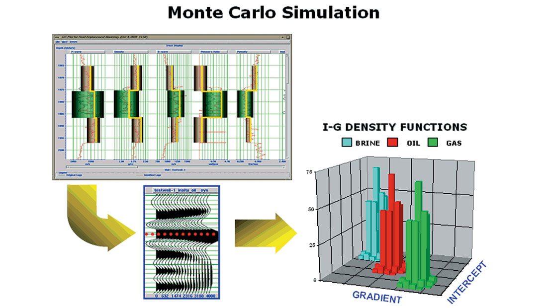
In this process, as shown in Figure 2, we first reduce the model to a manageable level of complexity – for example, by limiting the number of layers. Then we specify ranges and probability distributions for all the variables in the layers which affect the synthetic response. This, of course, is the hard part upon which all the rest hinges. Once we have probability distributions, standard statistical analysis theory allows us to generate a large number of “realizations” or possible models consistent with the assumed distributions. From each of the models, we calculate a synthetic and measure the resulting intercept and gradient. When we plot all of these values on a cross plot, we get something like the plot shown to the right of Figure 2. Instead of a single Brine point and a single Oil point, we now have a large cluster of points for each of the three fluid conditions which have been modeled. Theoretically each cluster represents the range of possible outcomes which are consistent with our probability distributions. The overlap between these clusters also tells us something about how well we can expect AVO analysis to distinguish between these conditions. (We will discuss this in more detail later.)

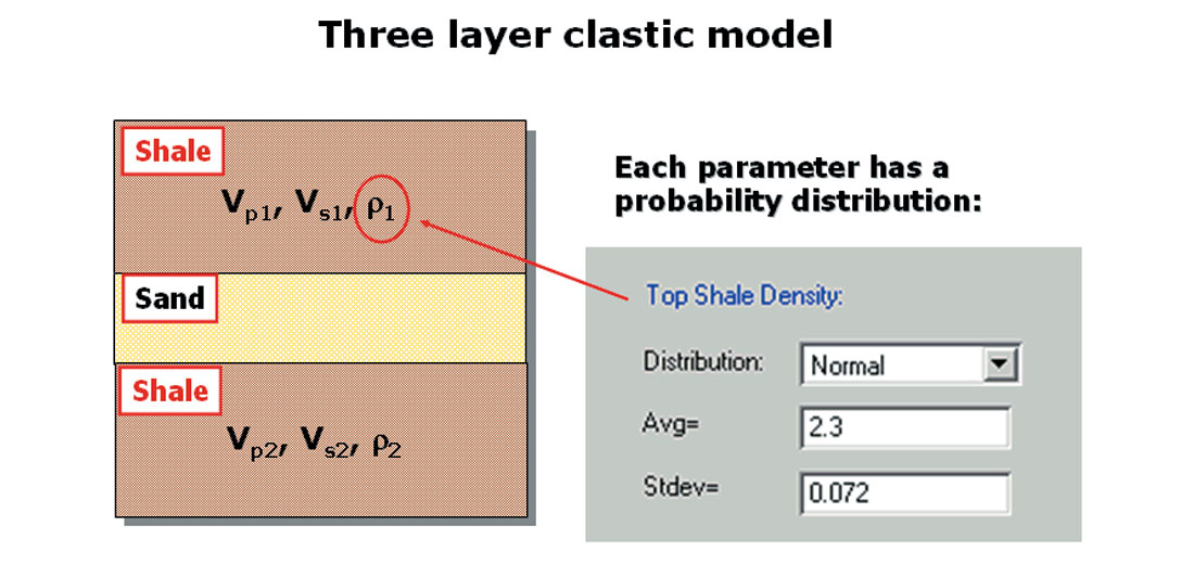
The target is assumed to be a sand layer, embedded between adjacent shales. The shales are characterized by the variables Vp, or P-wave velocity, Vs, or S-wave velocity, and density, where each of these variables is actually described by a probability distribution. The sand is characterized the large number of fundamental petrophysical parameters shown in Figure 4.

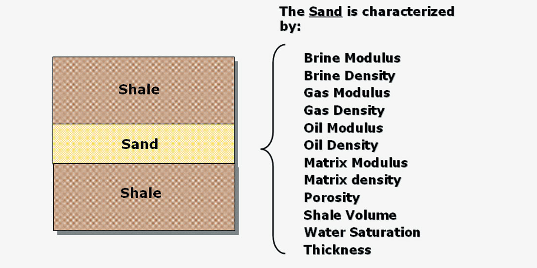
In theory, each of the parameters shown in Figure 4 may be described by a probability distribution, but in practice, many of the parameters are set as constants for the area. The very big task of determining reasonable distributions for these parameters is aided by analyzing trends from wells in the area, as shown in Figure 5.

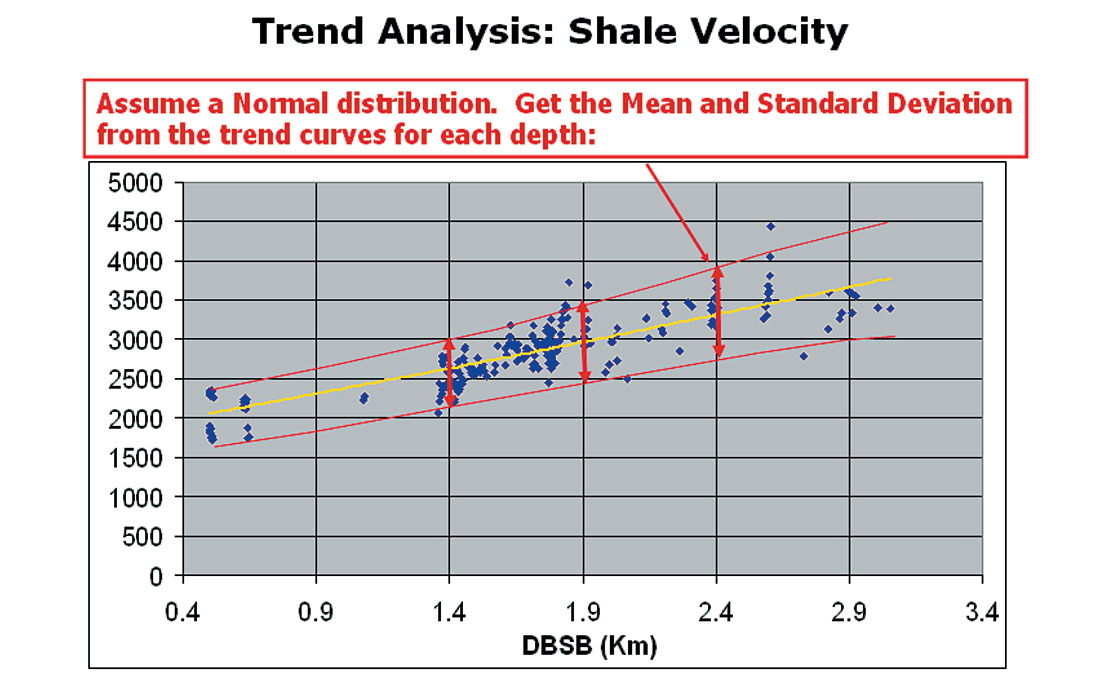
In Figure 5, P-wave velocity values for shale layers from a set of wells in the area have been collected and plotted as a function of depth. By fitting smooth curves through the points, we can get an idea of the average (Mean) and scatter (Standard Deviation) of shale velocities as a function of depth. Assuming a Normal Distribution, at selected depths, we can calculate the probability distributions needed.

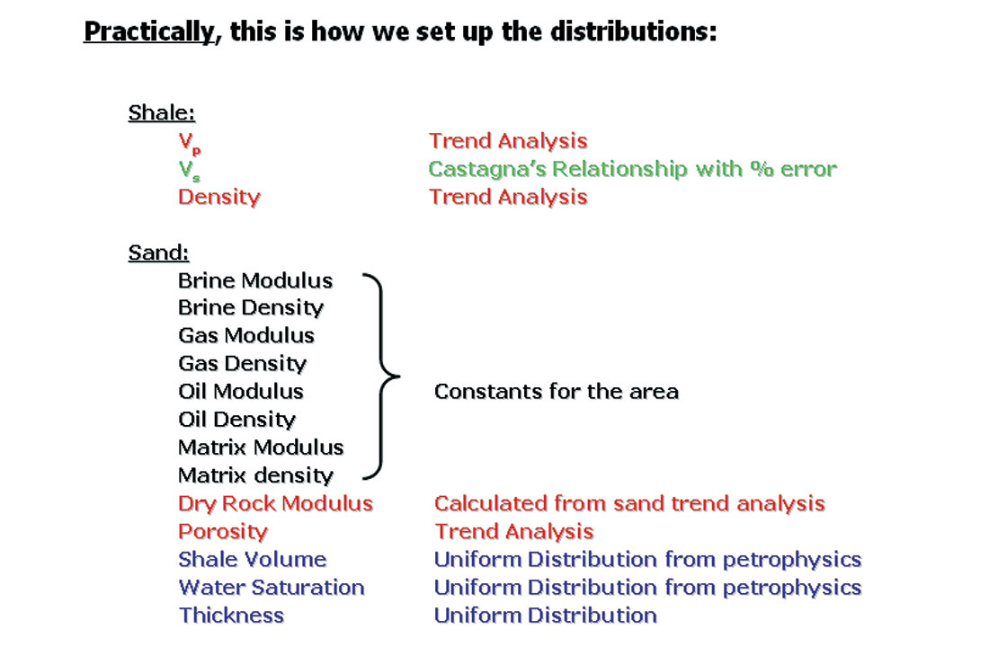
In practice, trend analysis from wells provides only a subset of the parameters which could be modeled. As seen in Figure 6, many other parameters are set as constants or modeled based on best-guess estimates and experience with the area.

Once the parameter distributions have been decided, it is a straight-forward computer task to perform the Monte-Carlo simulation. This process creates a large number of “realizations”. Each realization is a complete three layer model, with some specific value for each of the parameters. The relative occurrence for any particular parameter depends on the distribution we provided. For example, if the distribution for Vp, the P-wave velocity of the shale, has a very large scatter or standard deviation, then the resulting models will have a correspondingly large range of shale velocities, reflecting our lack of knowledge about this parameter.

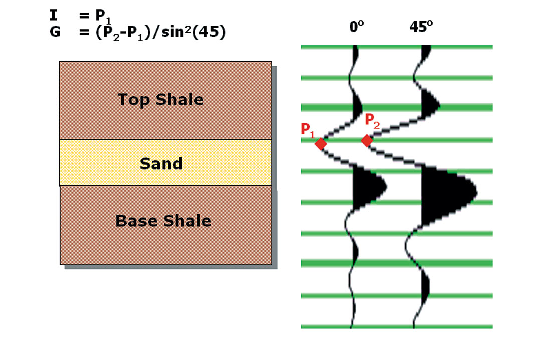
In order to compare these modeled results with real data, we need to calculate an attribute, which can be measured in the AV O analysis. In our case, we are using Intercept and Gradient, so each model is used to calculate a particular value of I and G, as shown in Figure 7:

From a particular realization or model, two synthetic traces are calculated at two angles. Note that this uses the seismic wavelet which is appropriate for the data set. From these synthetic traces, amplitudes are picked and the modeled values of I and G are calculated. Even though we are picking the amplitude at the top of the sand, the sand thickness affects the result because of interference from the wavelet at the base.

By performing a large number of simulations, we finally get a result such as that shown in Figure 8.

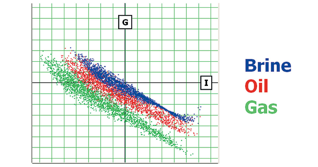
Figure 8 shows all the modeled points colour-coded, depending on whether the sand contains Brine, Oil, or Gas. From this figure , we can see the expected clustering of Brine points nearer the origin, with Oil and Gas points pushing further outwards. The figure also gives some idea of the relative separation of the clusters, indicating our ability to distinguish fluid properties using AVO analysis for this region.

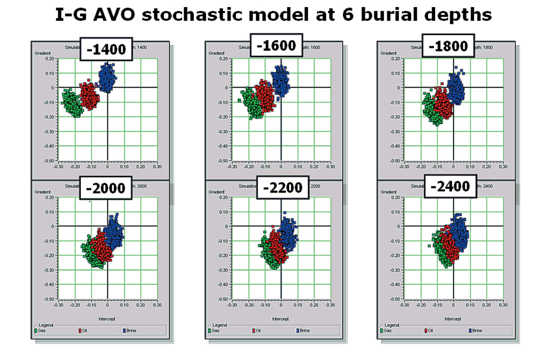
But this is just the modeled result at a single burial depth. By using the trend analysis, we can expect the parameter distributions to change with depth, resulting in a movement of the clusters, as illustrated in Figure 9.

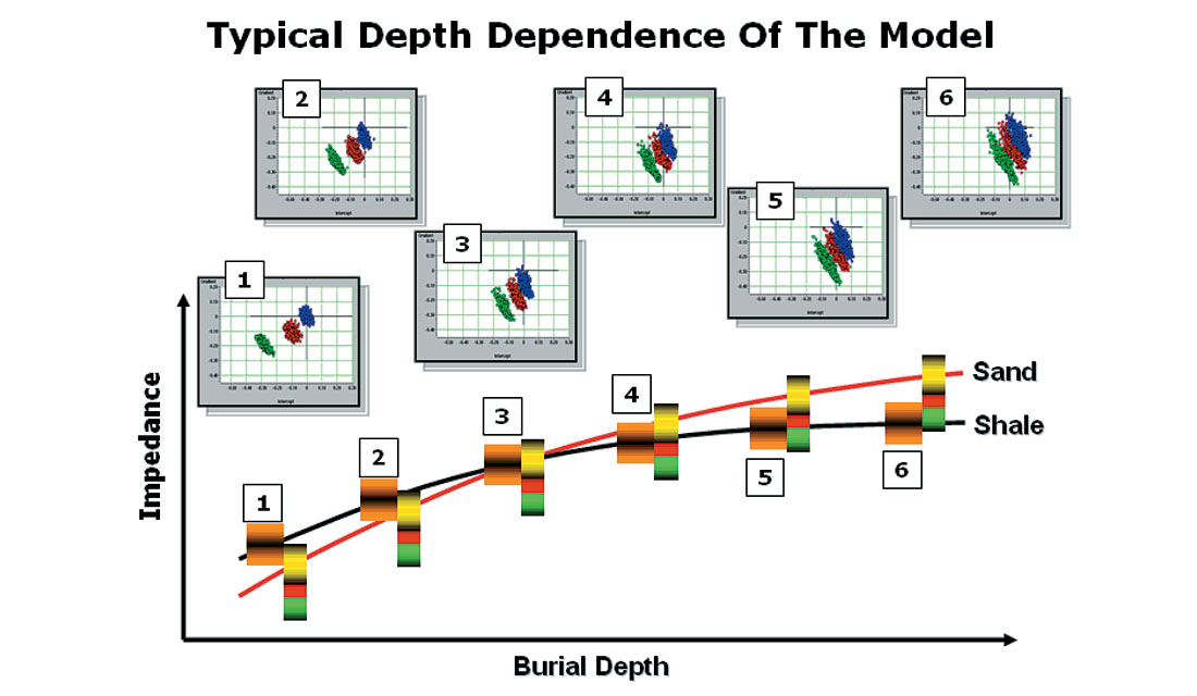
Figure 9 shows an example of how the distributions move around for a particular case where the average sand and shale impedance t rends cross. At point 1, for example, where the sand impedance is lower than the shale impedance, the corresponding cross plot shows typical Class 3 AVO behavior. On the other hand, at point 3, where the trend lines cross, we get Class 2 AVO behavior. And finally, point 6 shows a Class 1 behavior. (For a discussion of the various AVO classes, refer to the original paper by Rutherford and Williams (1989)).

Another important aspect of the distribution plot is shown in Figure 10.

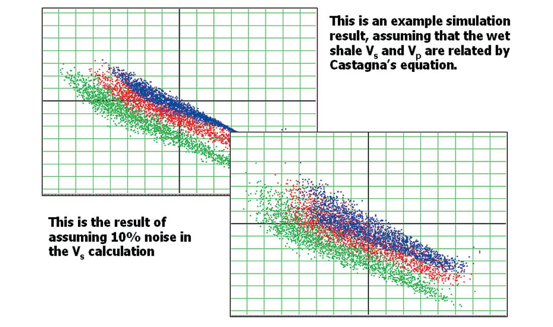
The two graphs from Figure 10 show distributions calculated from identical parameter sets, except that in the second distribution, the calculated shear-wave velocity for the shales was assumed to contain a 10% noise component. As a result, we see the distributions broaden and overlap, indicating a higher uncertainty in our ability to distinguish between the fluid properties using AVO analysis.

Finally, now that we have these clusters, how can we use them to evaluate AVO uncertainty numerically? The answer lies in a standard statistical algorithm, known as Bayes Theorem. This theorem answers the following question: given a particular cluster distribution, what is the probability that some new point (not on the clusters) belongs to each of the fluid types? An example of this calculation is shown in Figure 11.

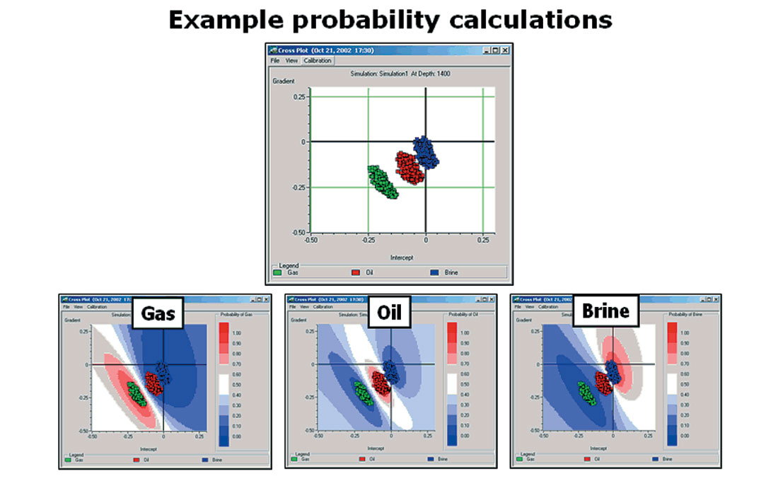
Figure 11 shows one particular cluster distribution, with three probability calculations, one for each of the fluid types. In this figure red represents high probability, while blue represents low probability. As expected, the high probability for, say, gas occurs very close to the green cluster of modeled gas values, and correspondingly for the other fluids. If all of the cluster distributions looked like this one, with very good separation, we would hardly need Bayes’ Theorem to tell us that. The more interesting, and usual, case is shown in Figure 12.

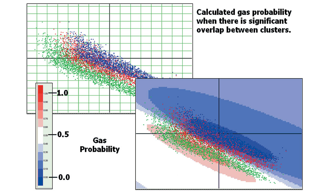
In the case shown in Figure 12, because of the overlap between the clusters, the area where there is a high gas probability is quite narrowly defined, and even at its best, the highest probability is around 70%. This means we can only be 70% sure we have gas – even if we measure a real data point directly on one of the green points. This shows the importance of Bayes’ Theorem to evaluate not only the location of the clusters, but their degree of overlap as well.

Calibrating to the Real Data

What we have achieved so far is that we can generate probability distributions in the Intercept/Gradient cross plots, based on probability distributions from the basic petrophysical parameters. This is already very useful because it allows us to estimate how well AVO should work in an area, if all the conditions are ideal.

The next step is to use these probability distributions to analyze our real data results. The idea is summarized in Figure 13.

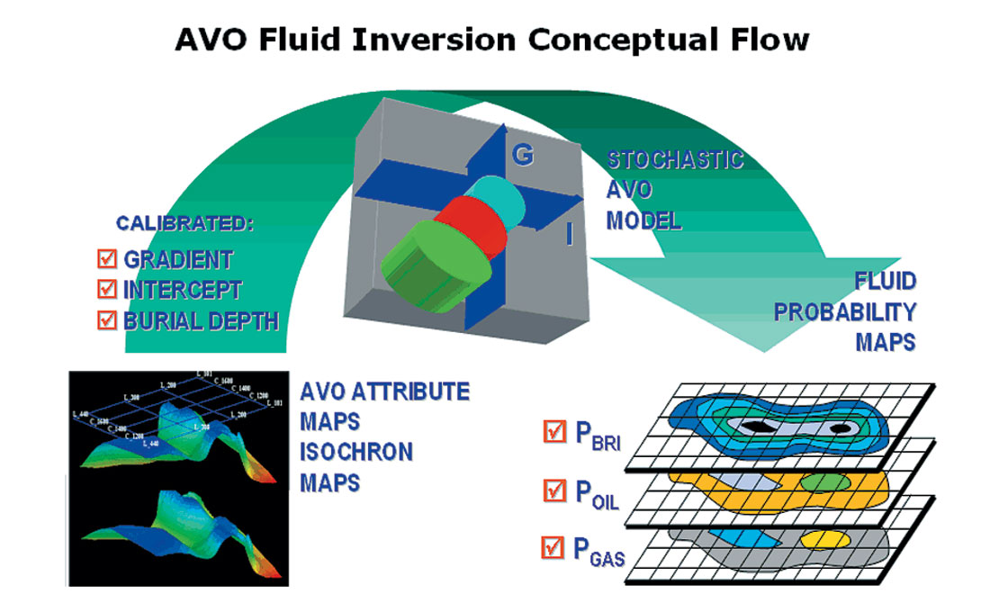
In Figure 13, the real data shown in the bottom left is a set of maps of Intercept and Gradient from a 3-D volume. Since we are dealing with depth trends, we may also need a map of burial depth. By comparing these maps with the stochastic models, we hope to generate Fluid Probability Maps, e.g., Probability of Gas.

In theory, this is very easy. For each point on the input maps, we create an Intercept/Gradient pair, find its location on the stochastic model cross plot, and read off the probability generated by Bayes Theorem. Unfortunately, there is a little catch: the real data values are not scaled properly. This is because conventional AVO software does not extract the actual Intercept and Gradient as defined by the Zoeppritz equations, but gives an arbitrarily scaled version of these numbers, depending on the scaling of the input seismic data. In addition to an overall scaling factor, there may also need to be an offset-dependent scaling to fix up processing problems or artifacts. We need to determine these scalers before comparing the real data values with the model values.

There are many possibilities for doing this calibration between the real and model data. For example, synthetic traces could be compared with the real traces and scalers found that way. A second possibility, which we use here, is to calibrate known locations on the attribute maps, as shown in Figure 14.

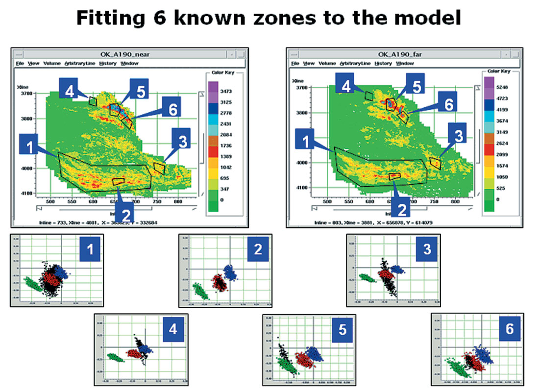
In Figure 14, we show two attribute maps from a 3-D prospect. The left map is the amplitude extracted at the top of the target event on the near-angle volume. The right map is the corresponding amplitude map from the far-angle volume. From these two maps, at each grid point, we calculate Intercept and Gradient. We also show on the maps, six zones which have been defined for various reasons. The six cross plots at the lower portion of the figure are the cross plots generated from the data in each of the six zones. On these cross plots, the black dots correspond to the real data Intercept/Gradient pairs, while the coloured points are the clusters calculated by stochastic modeling.

To perform the calibration between real and model cross plot values, we define two scalers this way:

I_MODEL = S_GLOBAL *I_REAL

G_MODEL = S_GLOBAL *S_GRADIENT *G_REAL

The first scaler, S_GLOBAL, multiplies both the real Intercept and Gradient by the same number. This effectively accounts for the overall global mis-match between the real and model data. The second scaler, S_GRADIENT , multiplies only the real Gradient. This handles the possibility that processing or other problems have caused an amplitude imbalance between the near and far traces.

Operationally, the scalers are determined in such a way as to force the known calibration zones to fall on the desired clusters. For example, in Figure 14, we know that zones 2, 3, and 6 are oil wells, 5 is a gas well, and zone 4 is assumed to be wet. To arrive at Figure 14, we have already adjusted the two scalers by a combination of automatic and manual calibration to achieve a consistent overlay of all zones. We can now apply Bayes’ Theorem, using these scalers, to the entire data set.

Real Data Example

As a real data example, we will show the application of this procedure to a 3-D data set from West Africa. The data set has been processed to produce a Near Angle Stack, containing incidence angles from 0 to 20 degrees and a Far Angle Stack, containing angles from 20 to 40 degrees. A single inline from each of the stacks is shown in Figure 15.

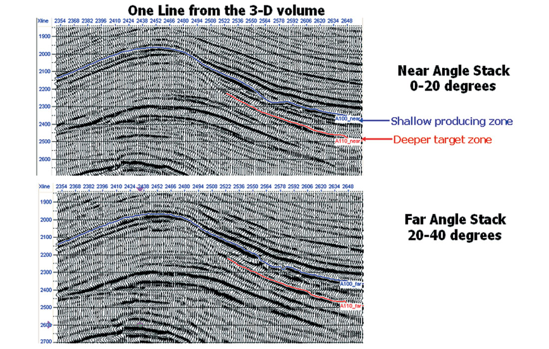
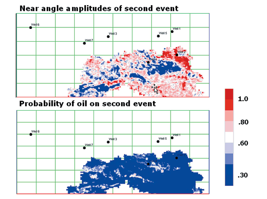
There are seven producing oil wells which tie the volume and produce from the shallow formation called “A100” on Figure 15. The object is to perform stochastic simulation using trends from the producing wells, calibrate to the known data points, and evaluate potential drilling locations on a second deeper formation, called “A110” on Figure 15.

Using the shallow formation horizon, amplitude maps were extracted at the seismic trough which is assumed to be the top of the productive sand. These maps are shown in Figure 16. Six of the oil wells are also displayed on this figure. We can see a significant increase in amplitude from near to far angles over a large channel-like region.

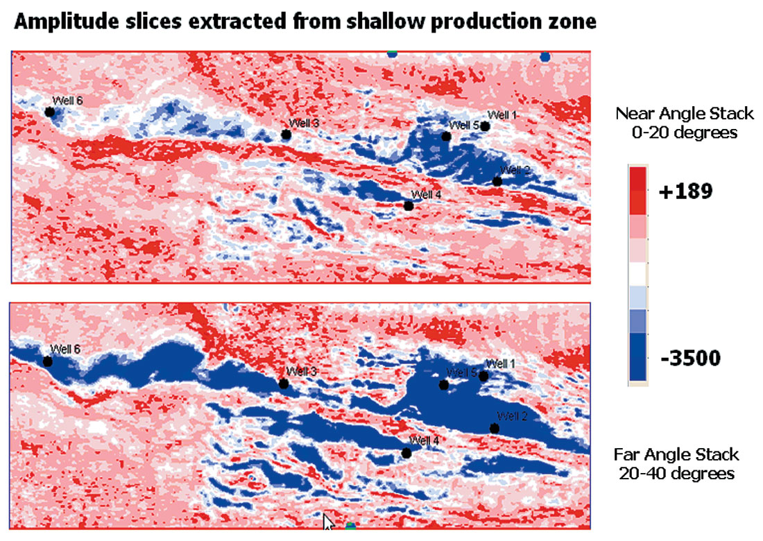
Figure 17 shows an example of the trend analysis which was performed on the wells to determine probability distributions. This figure shows the P-wave velocity from sand layers extracted from the wells, along with the interpreted trend lines. Using similar trend analyses for the sand and shale velocities and densities, as well as the porosity trend analysis, parameter distributions were established at 6 burial depths.

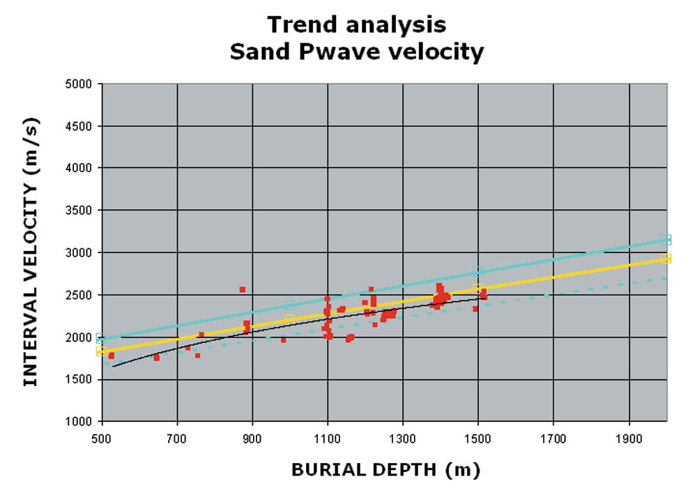
Figure 18 shows the result of stochastic modeling at the 6 burial depths, using the parameters established by trend analysis. As discussed previously, we can see a gradual shifting of the clusters from a clearly Class 3 behavior at 1400 meter depth to a class 2 behavior at 2400 meter depth.

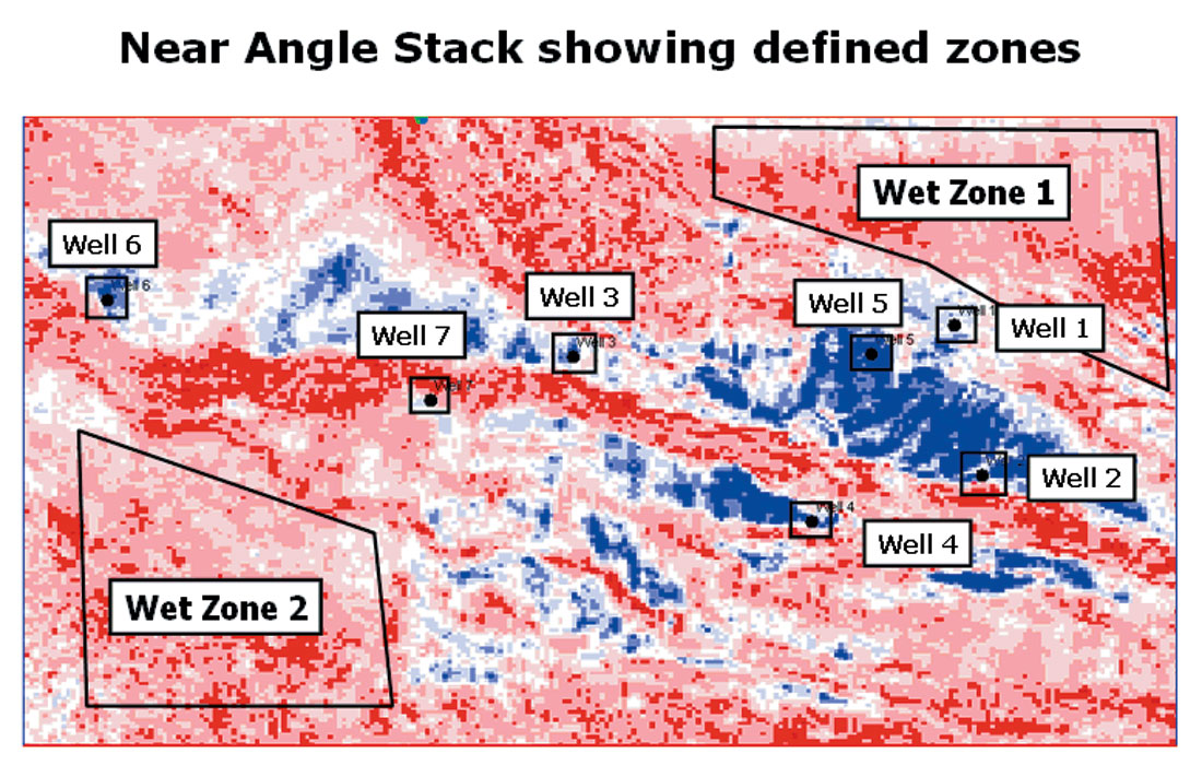
In Figure 19, we have selected zones around the well locations which we will use for calibration. In addition, we have selected two large zones, which we consider to be wet. These are labeled Wet Zone 1 and Wet Zone 2 on Figure 19, and are in the northeast and southwest corners of the map, away from the oil well locations.

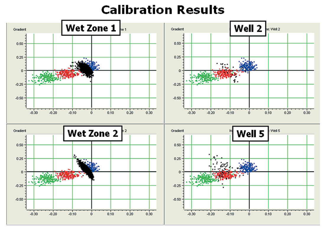
After manually adjusting the scaling parameters, Figure 20 shows the resulting calibration at four of the selected locations. As hoped, both wet zone data points fall reasonably well on the brine cluster, while the points from two of the oil wells fall on the oil clusters. The results for the other well locations were similar.

Using the calibration scalers in conjunction with Bayes’ Theorem, we produced the oil probability map shown in Figure 21. We can see that the highest probability is around 80%, even where the known oil wells are located. This reflects the uncertainty due to the overlap of clusters, especially at greater burial depths. We also note that the higher oil probability trends tie the production wells.

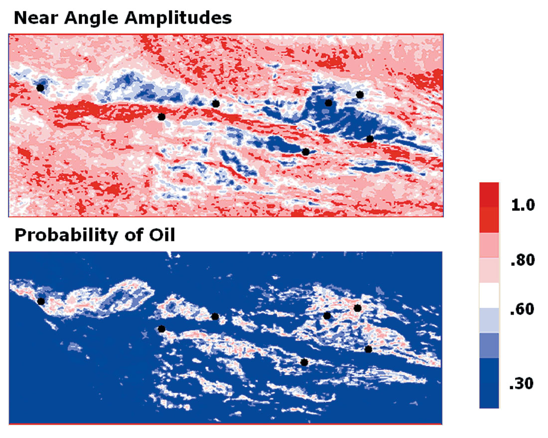
Finally, using the scalers and stochastic models derived from the shallow horizon, we apply Bayes Theorem to the deeper target horizon. The result is shown in Figure 22. The higher probability regions never exceed about 60%, which is probably reasonable, given the uncertainty of the entire AVO process. Effectively, we have generated one more tool for evaluating drilling locations on the second horizon, which contains its own measure of reliability.

Conclusions

AVO, like all geophysical measurements, is an uncertain tool. The level of uncertainty varies greatly, depending not only on the seismic data quality, but very much on the target lithology. To enhance the credibility of the AVO process, we need to be able to quantify that uncertainty.

One way of doing that is to create probability distributions for the underlying lithologic parameters, and derive the resulting distributions for the seismic-derived parameters. This allows us to calculate a probability or reliability for hydrocarbon predictions from the seismic data.

We must be very careful, though, to recognize that the value of those probabilities depends completely on the accuracy of the underlying distributions we create for the lithologic parameters. If we are going to provide uncertainty estimates along with our AVO predictions, those estimates must be reliable themselves.