Are there too many seismic attributes? Their great number and variety is almost overwhelming. How can one decide which ones to use? But it is not as bad as it looks. Throw away all the unnecessary attributes and what is left over is quite manageable.
It’s easy to identify unnecessary seismic attributes. Just review your attributes in the light of these common-sense principles:
- Seismic attributes should be unique. You only need one attribute to measure a given seismic property. Discard duplicate attributes. Where multiple attributes measure the same property, choose the one that works best. If you can’t tell which one works best then it doesn’t matter which one you choose.
- Seismic attributes should have clear and useful meanings. If you don’t know what an attribute means, don’t use it. If you know what it means but it isn’t useful, discard it. Prefer attributes with geological or geophysical meaning; avoid attributes with purely mathematical meaning.
- Seismic attributes represent subsets of the information in the seismic data. Quantities that are not subsets of the data are not attributes and should not be used as attributes.
- Attributes that differ only in resolution are the same attribute; treat them that way.
- Seismic attributes should not vary greatly in response to small changes in the data. Avoid overly sensitive attributes.
- Not all seismic attributes are created equal. Avoid poorly designed attributes.
Unnecessary attributes are thus duplicates, or they are obscure or unstable or unreliable, or they are not really attributes at all. Look first for duplicate attributes, the most numerous kind of unnecessary attribute. Many basic seismic properties, particularly amplitude, frequency, and discontinuity, are quantified through multiple seismic attributes variously computed.
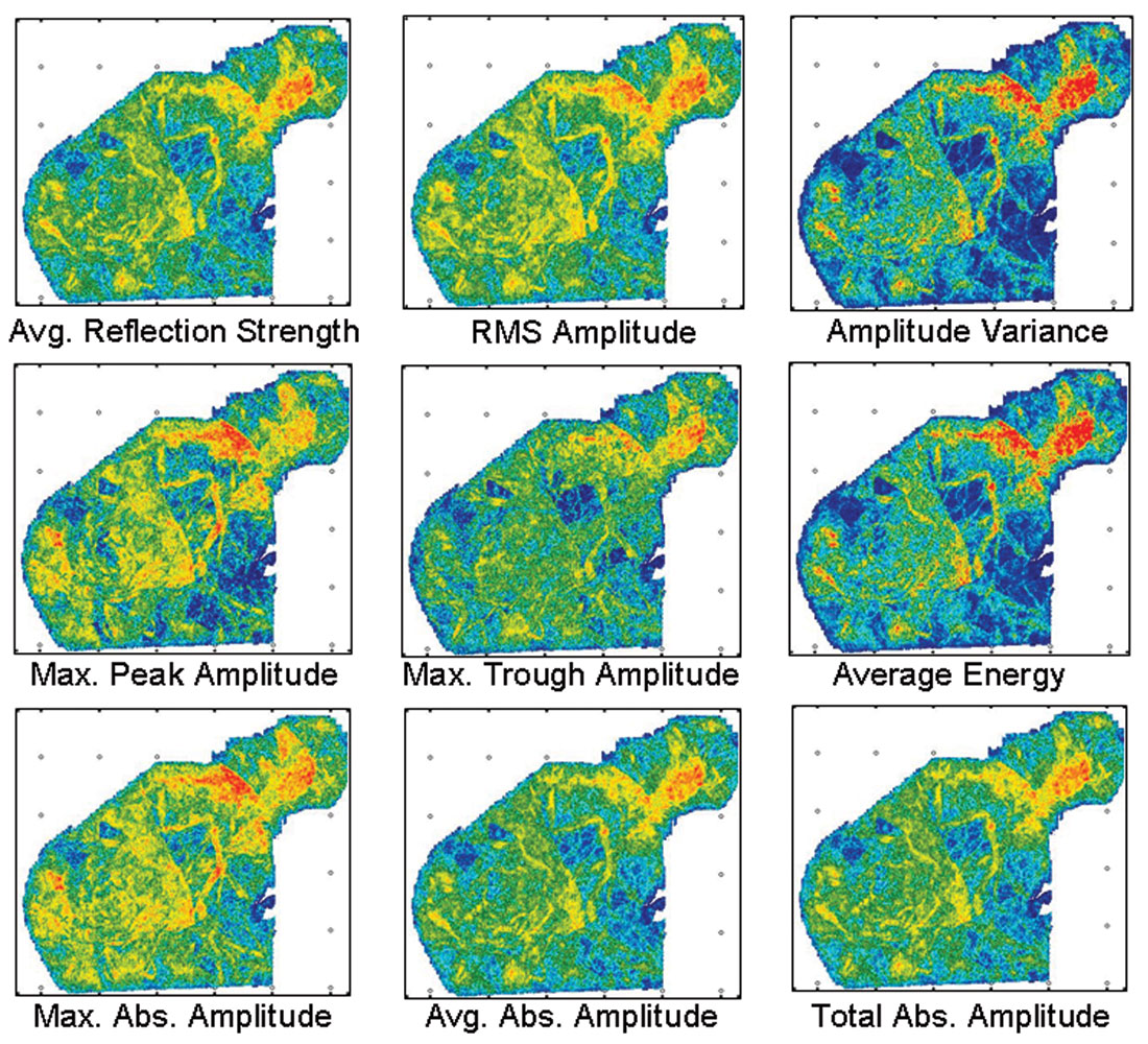
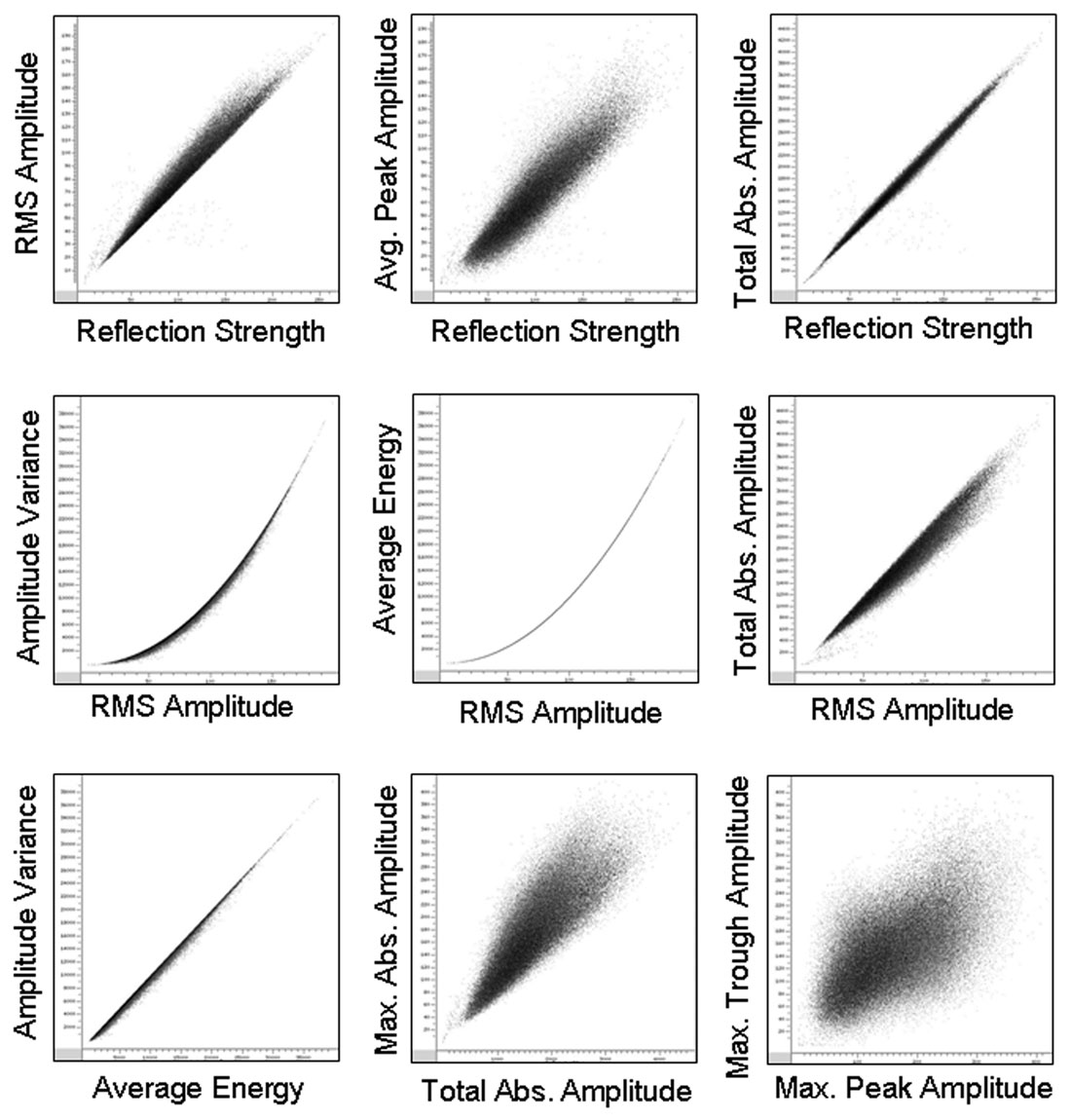
Consider the most important seismic property, amplitude. Figure 1 compares nine common amplitude attribute maps. These maps are all similar. Crossplots between them reveal fairly linear or quadratic relationships demonstrating that they contain nearly the same information (Figure 2). Rarely are the differences between these attributes important, and rarely is anything gained by using more than one. Average reflection strength nearly always suffices.
You may prefer average energy because it exhibits more contrast than reflection strength. Use it, but recognize that average energy has exactly the same information as RMS amplitude and almost the same as reflection strength. Its greater contrast is due only to how it presents the information. Perhaps also you want to use the maximum amplitude attribute because in your application it has useful meaning, and the differences between average reflection strength and maximum amplitude are significant – if you truly know what they mean.
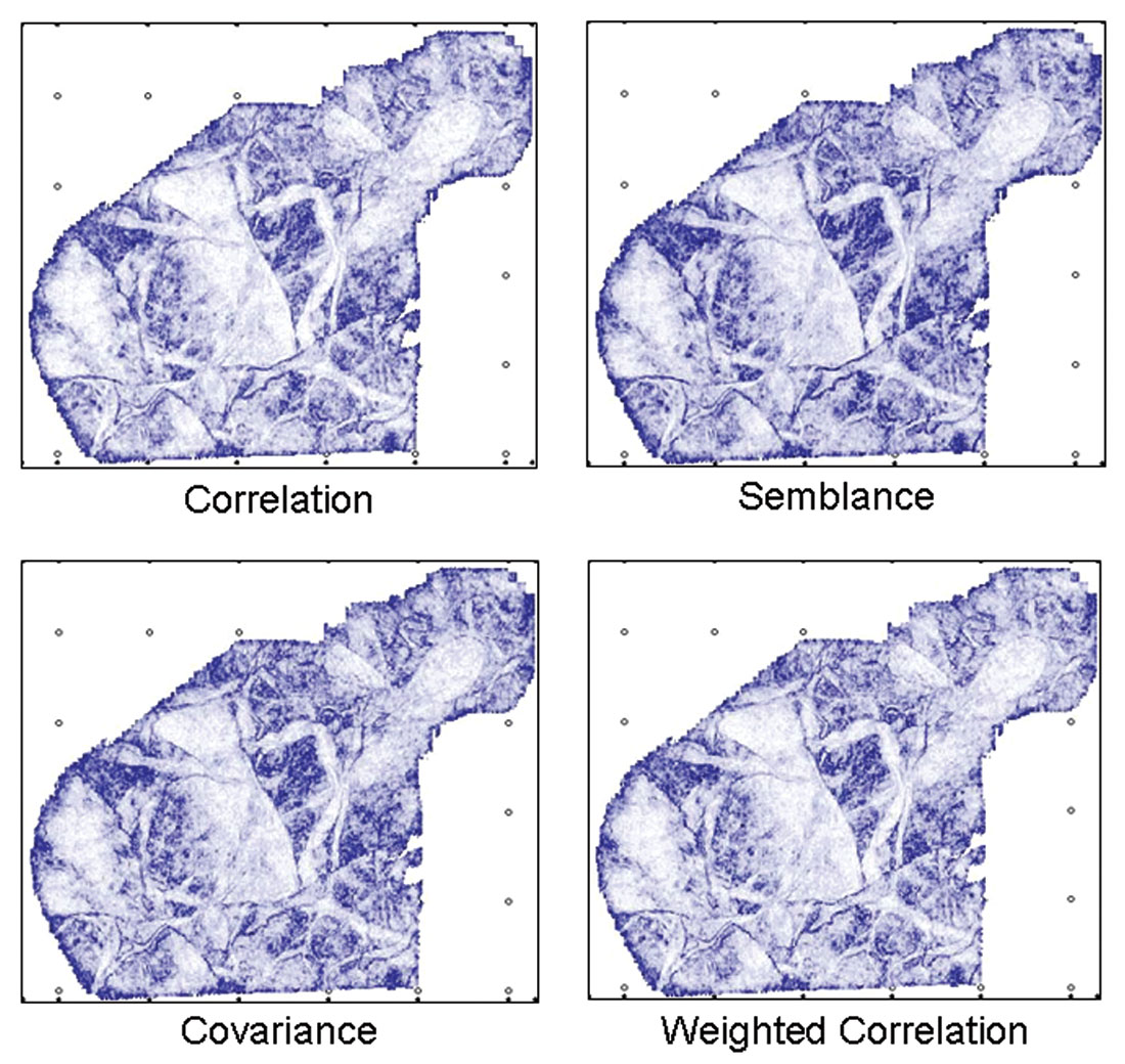
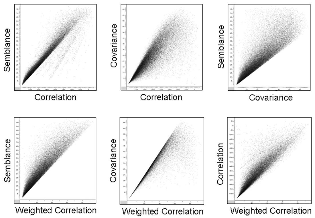
Take a more involved seismic property, discontinuity. Figure 3 compares four common discontinuity attributes based on correlation, semblance, covariance, and weighted correlation. Their crossplots are given in Figure 4. Despite significant computational differences and enthusiastic claims to the contrary, these four discontinuity attributes are so nearly the same that it doesn’t matter which one you use.
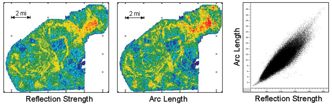
Many duplicate attributes masquerade as unique measures. Arc length is one of these. It is driven by both amplitude and frequency, but amplitude usually dominates to the extent that it resembles reflection strength (Figure 5). You probably don’t need it. Actually, you really don’t need it – arc length is nonsense. Defined as the length along the wiggles of a seismic trace in amplitude-time space, it has no useful meaning because amplitude and time are unrelated. Discard it.
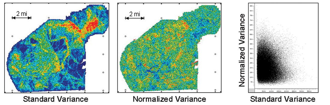
Amplitude variance also masquerades as a unique measure. Intuitively it should be unique, or at least much different than amplitude attributes such as reflection strength. But for zero mean data a standard variance equals the average energy, which is the square of the RMS amplitude, which is a close approximation to reflection strength. As a result, amplitude variance derived directly from seismic data resembles most amplitude attributes (refer to Figures 1 and 2).
An effective amplitude variance attribute can be defined as the variance of the reflection strength normalized by the average reflection strength. This normalized variance is different than amplitude and noisier than standard variance (Figure 6). Whether it is also useful must be determined empirically.
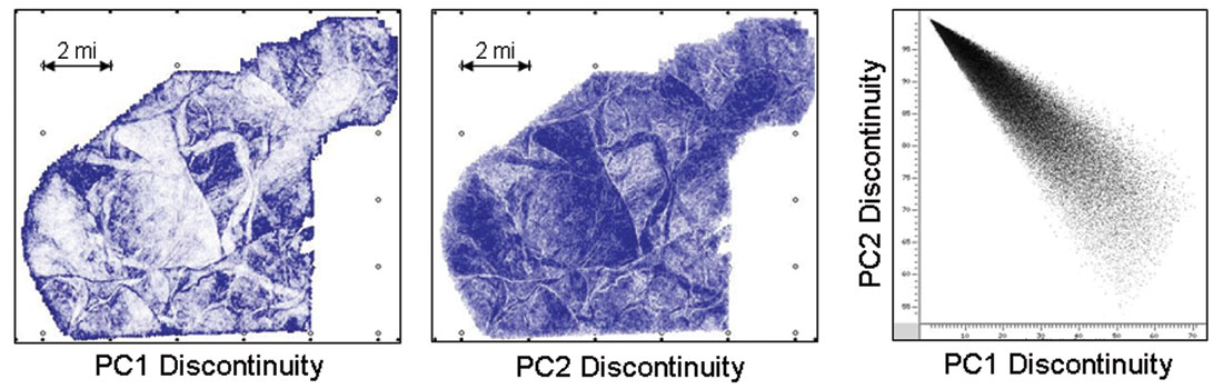
Attributes based on principal components often masquerade as independent measures. While principal components are naturally independent, normalized principal components tend to be well correlated. Figure 7 shows two seismic discontinuity attributes, one computed from the normalized first principal component, PC1, and another computed from the normalized second principal component, PC2. These look like mirror images of each other. A corresponding attribute based on the third principal component, PC3, resembles a fuzzy version of PC1. Ratios of principal components, such as the Karhunen-Loeve signal complexity (what does that mean?), can also look like PC1 and PC2. These principal component attributes all show the same picture. Keep PC1 and discard the others.
Further muddying the waters, some attributes have duplicate names. Reflection strength, trace envelope, and instantaneous amplitude are the same attribute. Covariance discontinuity, eigen-structure discontinuity, and the normalized first principal component, PC1, are the same attribute, which initially was called “Amoco C3.” Response attributes are also called wavelet attributes. The quadrature trace and the imaginary trace are the same – but this is a poor example. The quadrature trace is just a 90° phase rotation and is not an attribute since it does not subset the information.
Some attributes are more than similar, they are essentially identical. Identical attributes contain exactly the same information and differ merely in how they present this information. As already noted, RMS amplitude and average energy are identical. Other identical attributes include instantaneous phase and cosine of the phase, and dip-azimuth (reflection dip combined with reflection azimuth) and shaded relief. Choose the one you prefer and discard the other.
Cosine of the phase is not only identical to instantaneous phase, it is also nearly identical to a strong automatic gain (Figure 8). In fact, cosine of the phase is the ultimate automatic gain, completely removing all amplitude contrasts. Treat it more as a process than as an attribute.
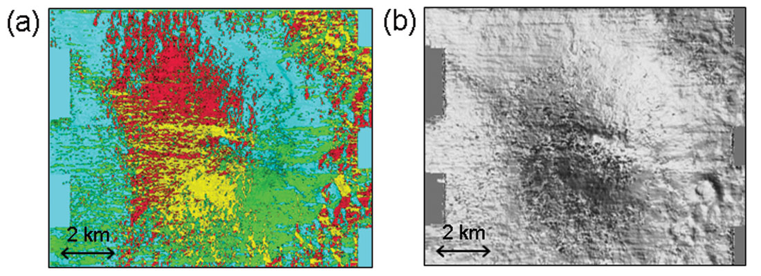
Though dip-azimuth and shaded relief are identical attributes, they look quite different (Figure 9). Dipazimuth combines reflection dip and reflection azimuth through a circular two dimensional colorbar for which azimuth controls the hue and dip controls the intensity. Shaded relief combines reflection dip and azimuth to simulate the shading of illuminated reflections, for which a gray-scale colorbar suffices. You don’t need both.
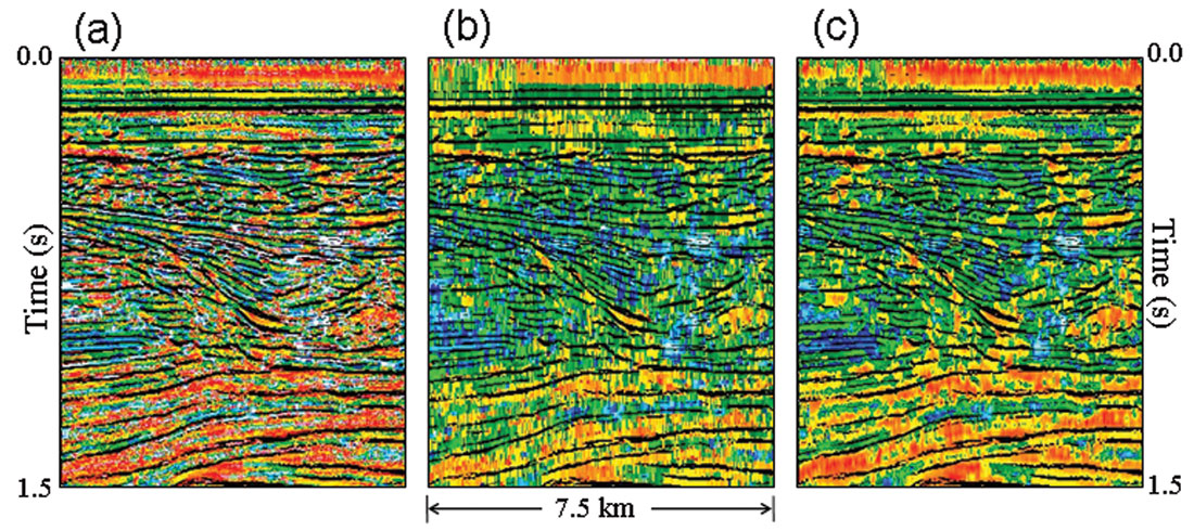
Attributes that lack clear and useful meaning might well be labeled useless. Such attributes are more common than you would think. Arc length and the Karhunen-Loeve signal complexity are useless attributes. Average instantaneous phase is another useless attribute. The more instantaneous phase is averaged, the more predictable and the more worthless the result: zero. Average unwrapped instantaneous phase is scarcely better. The “slope of the instantaneous frequency” may have clear mathematical meaning (or may not), but its geological meaning is so obscure that it is useless. Response phase and response frequency are also useless if you insist that they describe the seismic source wavelet as advertised. They succeed only in the absence of noise or reflection interference. Simply put, they succeed only in the absence of real data. You can use these attributes empirically, of course, recognizing what they really record. Response phase records the apparent phase of reflections, composite or solitary, at envelope peaks, and helps in tracking events. Response frequency acts like a nonlinear filter for instantaneous frequency, producing a cleaner attribute free of spikes and negative values. This has utility, but a weighted average frequency is better because it offers the same benefits plus it is smoother and has simpler meaning (Figure 10).
Changing the resolution of an attribute does not change its nature. An attribute remains inherently the same whether computed in a short window or in a long window. This is obvious for attributes like RMS amplitude and energy half-time, but it is also true, though not obvious, of instantaneous frequency and weighted average frequency. They are really the same frequency attribute with different resolution. You might reasonably use both to investigate targets with different resolution, but recognize they are the same attribute.
Weighted average frequency can be computed either in the time domain as weighted average instantaneous frequency, or in the frequency domain as weighted average Fourier spectral frequency. With appropriate weights, these completely different methods produce exactly the same results. Similarly, bandwidth can be quantified as a spectral variance either in the time-domain or in the frequency domain. Some multi-dimensional attributes, such as azimuth, dip, or dip variance (a measure of reflection parallelism), can also be generated in either domain. Because these attributes are the same in either domain, it is pointless to compute them in both domains. Not all spectral attributes are so flexible. Spectral kurtosis, for example, must be computed in the frequency domain, but as it has no inherent geological or geophysical meaning, you probably don’t need it.
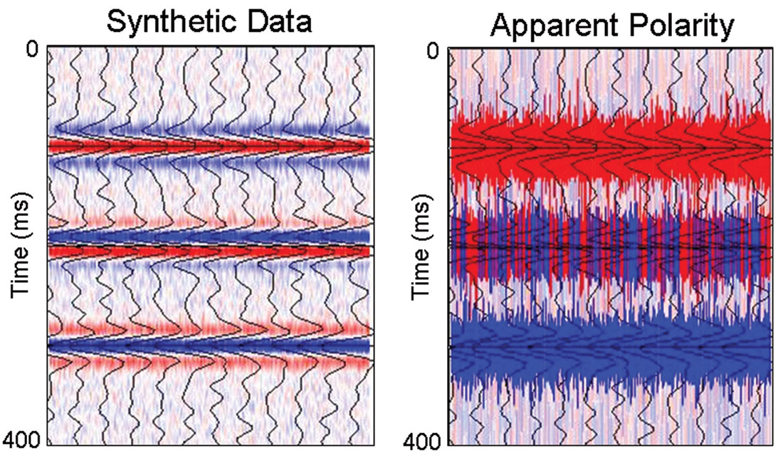
Attributes that are sensitive to small perturbations in the data are unstable. Apparent polarity is an example. It is defined as the sign of the seismic data at envelope peaks scaled by the envelope peak and held constant in each interval around a peak. This works fine for clean zero-phase data free of reflection interference, but it is ambiguous for thin-bed reflections, which have an apparent phase of around 90°. Figure 11 shows this for simple synthetic data. As long as the reflections don’t interfere, apparent polarity is correct, but where they do interfere, apparent polarity flips randomly from trace to trace. The same problem occurs on real data. Discard apparent polarity and use response phase instead. Attributes that count the integral number of peaks or troughs in an interval are also unstable, as they are sensitive to small changes in interval definition. The details shown by these attributes cannot be trusted; avoid them.
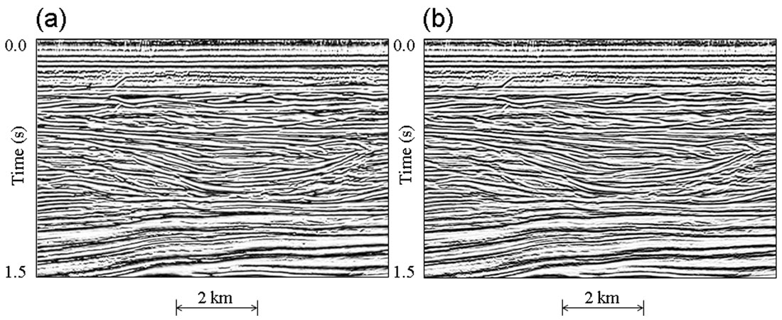
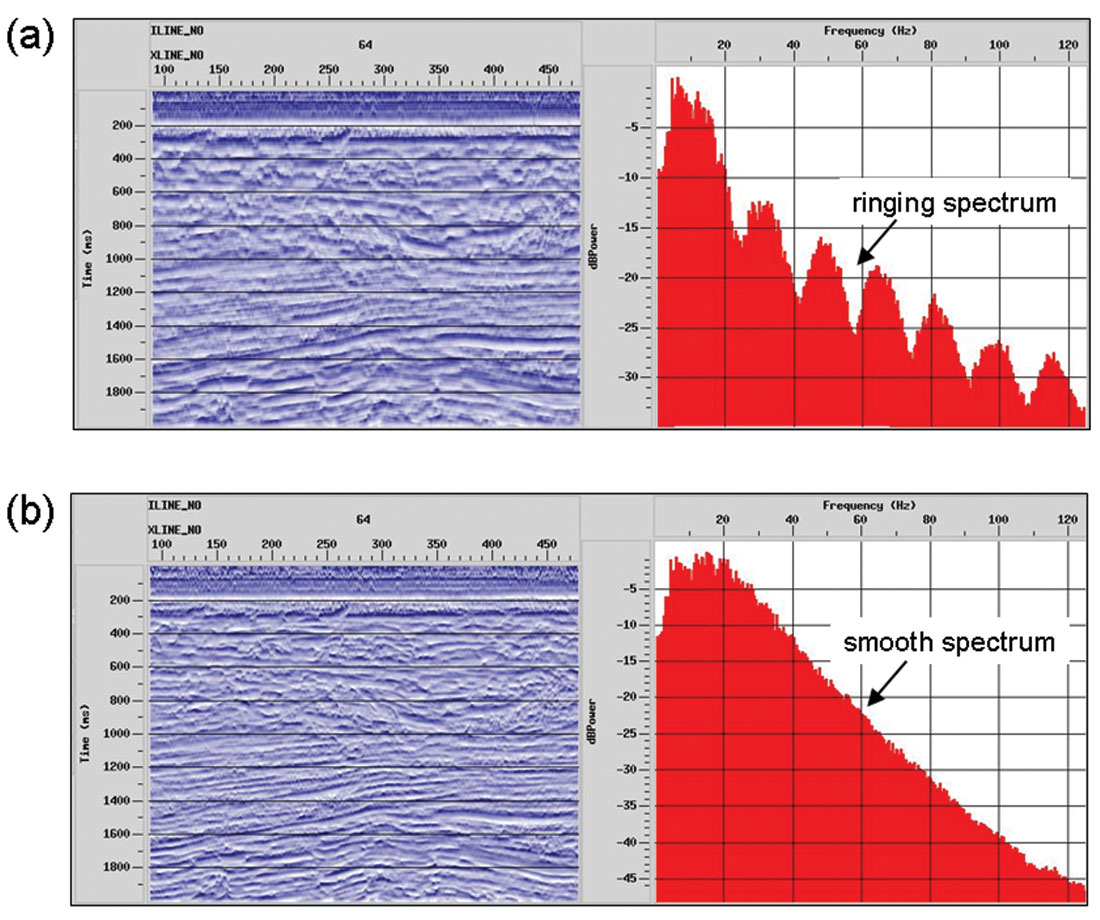
Beware of differences between programs for generating seismic attributes. Aside from incorrect algorithms, which especially plague instantaneous frequency, the same attribute produced by competing programs can differ substantially due to implementation details. One such detail regards the windowing, which is the way an algorithm selects seismic data from an interval. Attributes are filters, and like any filter they should employ tapered windows to reduce Gibb’s effects. Non-tapered or “boxcar” windows are nonetheless widely used. Figure 12 compares the effect of a boxcar window with that of a tapered window of the same length in the computation of energy half-time. The boxcar window gives rise to banding in the time domain and ringing in the frequency domain, which are the Gibb’s effects. The tapered window produces a sharper image and a smoother power spectrum. Where possible, avoid attributes with ringy spectra.
Energy half-time is a measure of amplitude change. Use it in this sense. Optimistic descriptions that suggest it to be a lithologic indicator are wrong.
I could review many more seismic attributes, including waveform, spectral attributes, curvature, AVO attributes, and others, to weed out the unnecessary ones. But I have made my point: there are too many duplicate attributes, too many useless attributes, and too many misclassified attributes. This breeds confusion and makes it hard to apply attributes effectively. Reduce your attributes to a manageable subset. Discard duplicate and dubious attributes, prefer attributes that make intuitive sense, understand resolution, distinguish processes from attributes, and avoid poorly designed attributes. Tables 1 and 2 summarize these ideas. Table 1 lists all the attributes mentioned here, while Table 2 lists only those worth keeping. Table 1 looks impressive but is too confusing to be helpful. In contrast, Table 2 is more honest and much clearer, and consequently is more useful.
Do you have too many seismic attributes? Throw away the ones you don’t need and your attribute analysis will improve.
| Amplitude | Phase | Frequency | Discontinuity | Miscellaneous |
|---|---|---|---|---|
| Table 1. A list of all the seismic attributes mentioned in this paper categorized by the properties that they measure. | ||||
| reflection strength | instantaneous phase | instantaneous frequency | correlation discontinuity | arc length |
| trace envelope | cosine of phase frequency | weighted average instantaneous | semblance discontinuity | energy half-time |
| instantaneous amplitude | apparent polarity spectral frequency | weighted average Fourier | covariance discontinuity | quadrature trace |
| RMS amplitude | response phase | response frequency | eigen-structure discontinuity (combined) | dip-azimuth |
| average or total absolute amplitude | average phase | spectral bandwidth | PC1 | shaded relief |
| maximum peak, minimum trough amplitudes | unwrapped phase | spectral frequency variance | PC2 | Karhunen-Loeve signal complexity |
| average energy, total energy | spectral kurtosis | PC3 | azimuth, dip | |
| standard amplitude variance | instantaneous frequency slope | Amoco C3 | dip variance | |
| normalized amplitude variance | parallelism | |||
| Amplitude | Phase | Frequency | Discontinuity | Miscellaneous |
|---|---|---|---|---|
| Table 2. The list of seismic attributes from Table 1 after ruthless clean-up. | ||||
| reflection strength | response phase | frequency | discontinuity | shaded relief |
| normalized amplitude variance | bandwidth | azimuth, dip | ||
| energy half-time (amplitude change) | parallelism | |||

Acknowledgements
I thank Seitel Data Ltd. for permission to publish the seismic data used in Figures 1 through 7, and I thank the Geological Survey of Denmark and Greenland, GEUS, for permission to publish the data used in Figure 9.


Join the Conversation
Interested in starting, or contributing to a conversation about an article or issue of the RECORDER? Join our CSEG LinkedIn Group.
Share This Article