Time-Frequency Polarization Analysis and Filtering

Introduction

Most of the “traditional” methods of polarization analysis and polarization filtering operate entirely in the time domain, or entirely in the frequency (or Fourier) domain. Unfortunately, both approaches have major limitations. Time-domain methods often have difficulty dealing with overlapping events that have different frequencies; and frequency-domain methods can run into trouble if events that have the same frequency occur at different times. The situation worsens if the events in question have different polarization properties. Conditions like these are of course epidemic in seismic data and, as a result, pure time-domain and pure frequency-domain techniques are inherently not very well suited to seismic processing. However, before the mid-1980s, these were the only methods available.

Jurkevics (1988) incorporated elements from both the time-domain and frequency-domain approaches to produce a mixed-domain technique. This led to the idea of using combined time-frequency representations, such as the Gabor transform and wavelet transforms, to alleviate the problems of the separate time and frequency domains. Since then, a number of multicomponent time-frequency techniques have been published in the literature. Examples include Lilly and Park (1995), Claassen (2001), Zanandrea et.al. (2003), and, more recently, Diallo et.al. (2005). Some of these methods focus entirely on polarization analysis, but others are invertible, and can be used for polarization filtering.

Where these methods are concerned, the issue is not one of technical validity, but ease of use, and practical implementation. Several of them require knowledge of specialized mathematics that is time consuming to learn. Others describe polarization in non-intuitive ways; for example, the orientation of the polarization plane may be described in terms of direction cosines, instead of strike and dip. With multicomponent trace analysis becoming more common in exploration geophysics, there is plenty of incentive to develop better techniques.

To that end, this paper describes a method of time-frequency polarization analysis and polarization filtering that is more intuitive than the others. Only the concepts are covered here. For a detailed description of the mathematics behind the technique, the reader is referred to Pinnegar (2006).

Elliptical elements

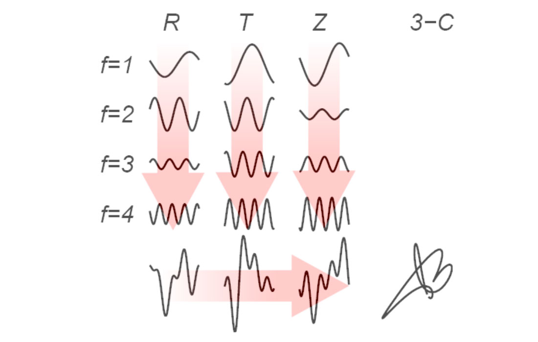
The basic idea is easiest to understand if we start with the Fourier decompositions of the separate components of a synthetic multicomponent trace, as depicted in Figure 1. Here, each column corresponds to a trace component (radial R, transverse T, or vertical Z). We know from Fourier’s theory that each trace component can be expressed as a superposition of sinusoids that have different frequencies. These sinusoids appear in the first four rows of Figure 1. Their amplitudes and phases, as functions of frequency, give the familiar Fourier amplitude and phase spectra of the trace components. The trace components themselves are shown in the bottom row. By combining these in 3-space, we obtain the whole trace, a hodogram of which is shown in the bottom right subplot.

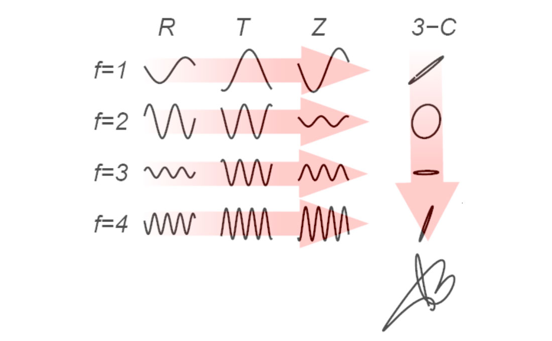
Alternatively, we can first consider the signal one frequency at a time, instead of one component at a time. At any particular frequency, there are sinusoidal contributions to the R, T and Z trace components, which, when combined, give elliptical motion in 3-space, as illustrated in Figure 2. (Another way of thinking of this is to recall that phase-shifted, time-dependent sinusoids, like those shown in Figures 1 and 2, basically behave like one-dimensional simple harmonic oscillators. Superimposing three of these that have the same frequency, but orthogonal directions of motion, is then equivalent to setting up the three-dimensional simple harmonic oscillator problem, whose solution gives elliptical particle motion in 3-space.) In the same way that the separate trace components are superpositions of sinusoids, the whole trace can now be thought of as a superposition of ellipses.

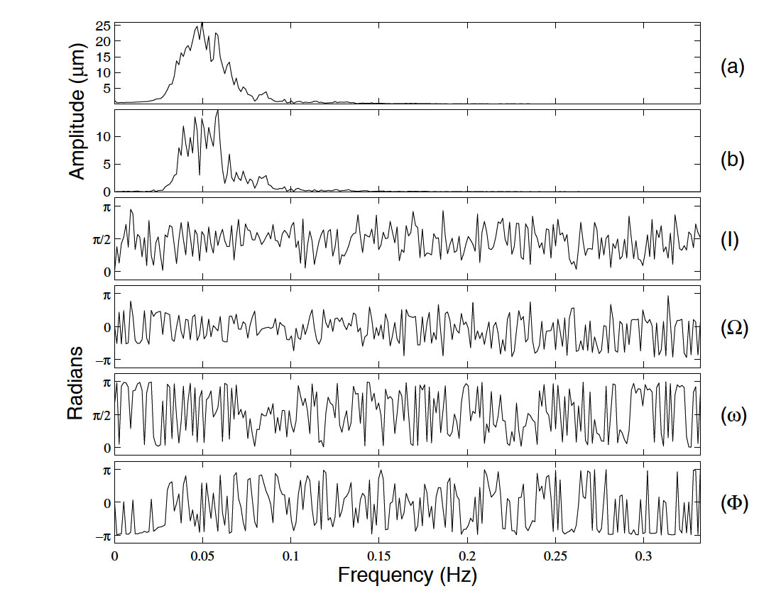
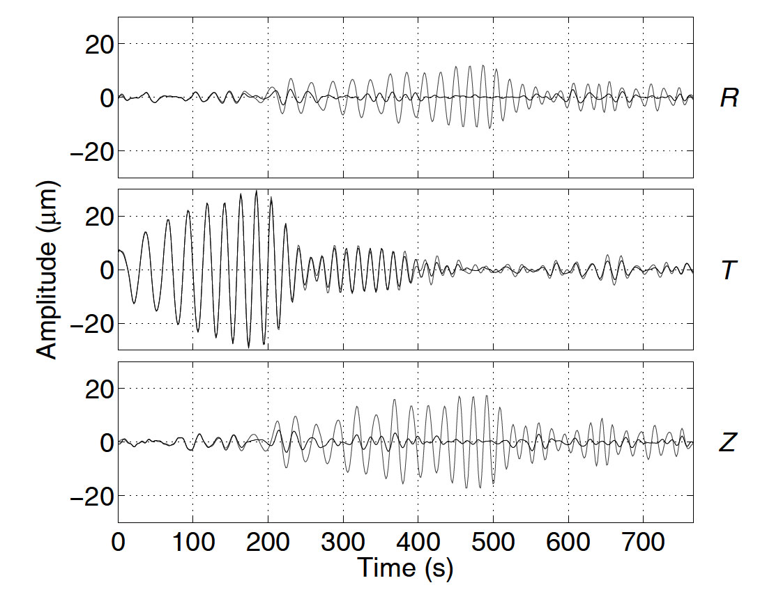
As a result, the Fourier amplitude and phase spectra of the separate R, T and Z trace components are replaced by a new system of Fourier spectra that describe these ellipses. Each ellipse is uniquely defined by six elliptical elements: the lengths of its major and minor axes; the strike and dip of its plane; the pitch of its major axis; and the phase of its particle motion. These elements describe the contribution of each frequency to the whole trace. As an example, Figure 3 shows the R, T and Z components for the surface-wave portion of an earthquake trace, and Figure 4 shows its Fourier elliptical-element spectra. The spectra of the major and minor axes have a familiar appearance, since these essentially replace the Fourier amplitude spectra of the separate trace components. The remaining four spectra all describe angles, so they tend to resemble the single-component Fourier phase spectrum (with similar problems for visual interpretation).

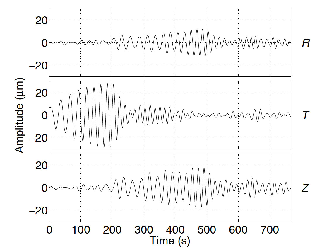
The elliptical-element spectra are invertible (i.e. they contain all the information that is needed to reconstruct the original trace) so, in principle, it should be possible to filter Figure 3 using the information in Figure 4. Unfortunately, this is easier said than done. The crux of the problem is that, as depicted in Figure 2, the three Fourier sinusoids that make up each ellipse have to have constant peak-to-peak amplitudes and constant phases. As a result, at any particular frequency, the contributing ellipse has to maintain the same size, shape, and orientation for the whole duration of the time series. Real signals, though, generally have highly time-dependent polarization properties. For example, the Love and Rayleigh phases shown in Figure 3 occur at different times, and have completely different polarizations, but lie within the same frequency band, and are therefore described by the same set of ellipses. In analogy with the one-component case, constructive and destructive interference between the different ellipses in the Love-Rayleigh band makes it possible for them to collectively describe Love wave motion at one time, and Rayleigh wave motion at another time. However, each individual ellipse will contain both types of motion, and is unlikely to closely resemble either as a result. This makes it just about impossible to use the known polarization properties of Love and Rayleigh waves to construct a signal-adaptive filter that would be able to (for example) remove one type of motion while retaining the other.

Time-frequency polarization analysis

Fortunately, there is a way out of this mess, which is to give the spectra of Figure 4 explicit time dependence by using a translating window to localize the Fourier spectra in time. Each function of frequency from Figure 4 now becomes a time-frequency representation, or TFR. (The TFR used by us is the Stockwell transform, which resembles a wavelet transform; however, other invertible TFRs, such as the short-time Fourier transform, can be used in its place if desired.) By using TFRs, we permit the ellipses that make up the trace to change with time, which gives a more robust technique that does not suffer from the problems described in the previous paragraph.

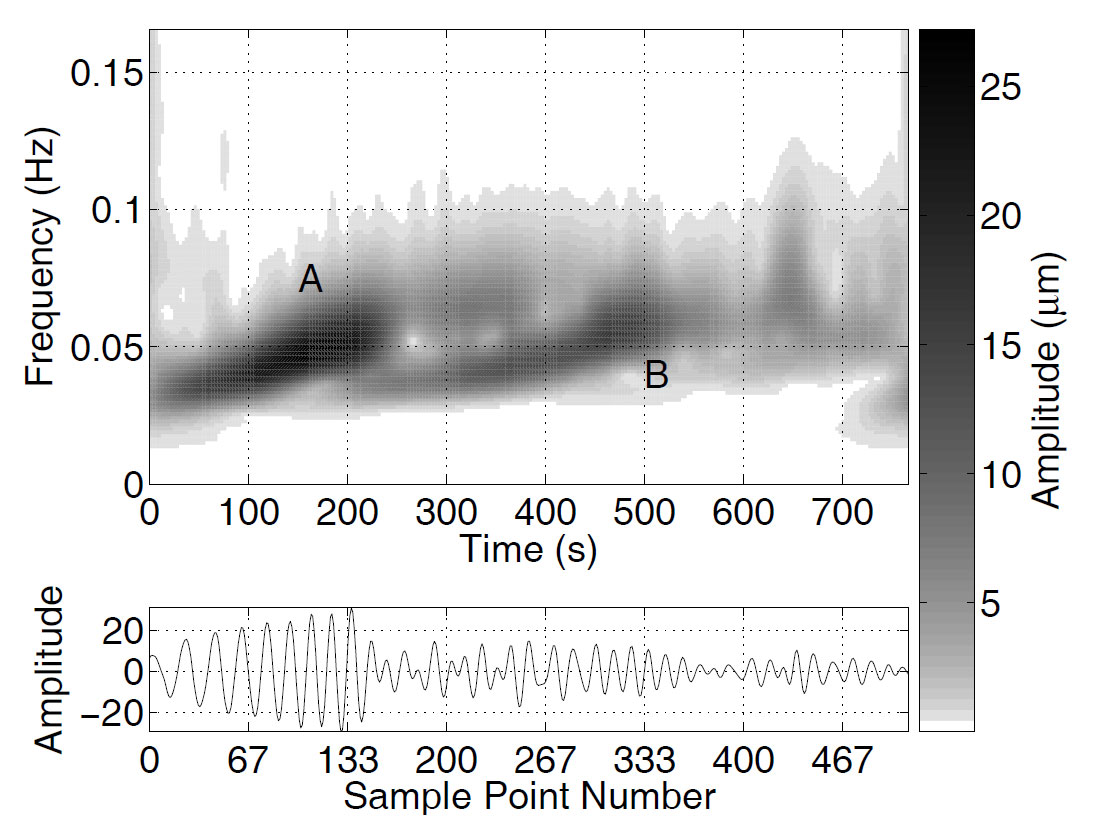
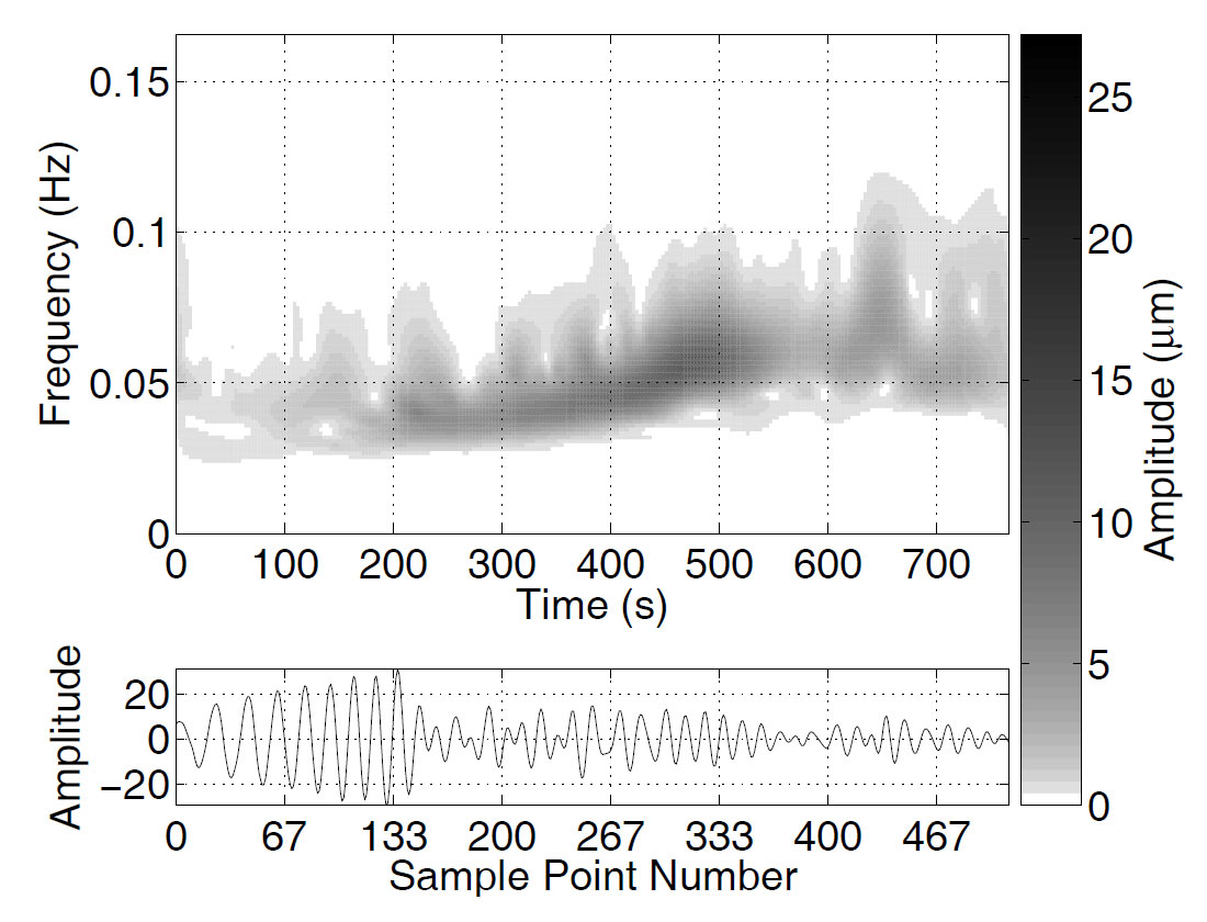
Figure 5 shows the major-axis TFR of the earthquake trace from Figure 3. Each column of Figure 5 represents a local spectrum, similar to the (a) and (b) spectra from Figures 3 and 4. The first large amplitude event (marked A) is the Love wave, and the second (marked B) is the Rayleigh wave. Both show obvious dispersive effects, with the higher frequencies arriving later. Comparing Figure 5 with the minor-axis TFR (Figure 6) clearly shows the differences in the polarization properties of the two phases. The Love wave has a small amplitude on Figure 6, a consequence of its nearly linear particle motion which has a very small minor axis. Turning to the Rayleigh wave, we find that its signature on Figure 5 has about 1.5 times the amplitude of the corresponding signature on Figure 6. Thus, for this trace, the Rayleigh wave has a major-to-minor axis ratio of roughly 3:2. (The minor axis must of course by definition always be smaller than the major axis.)

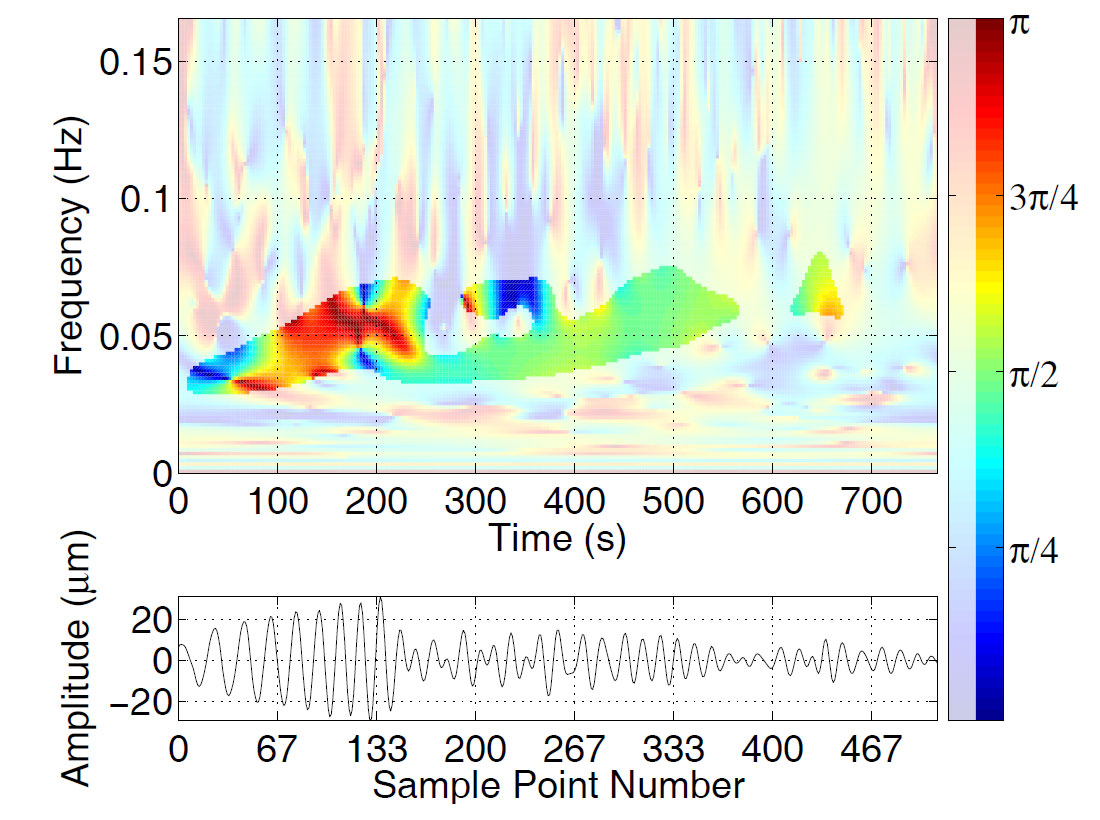
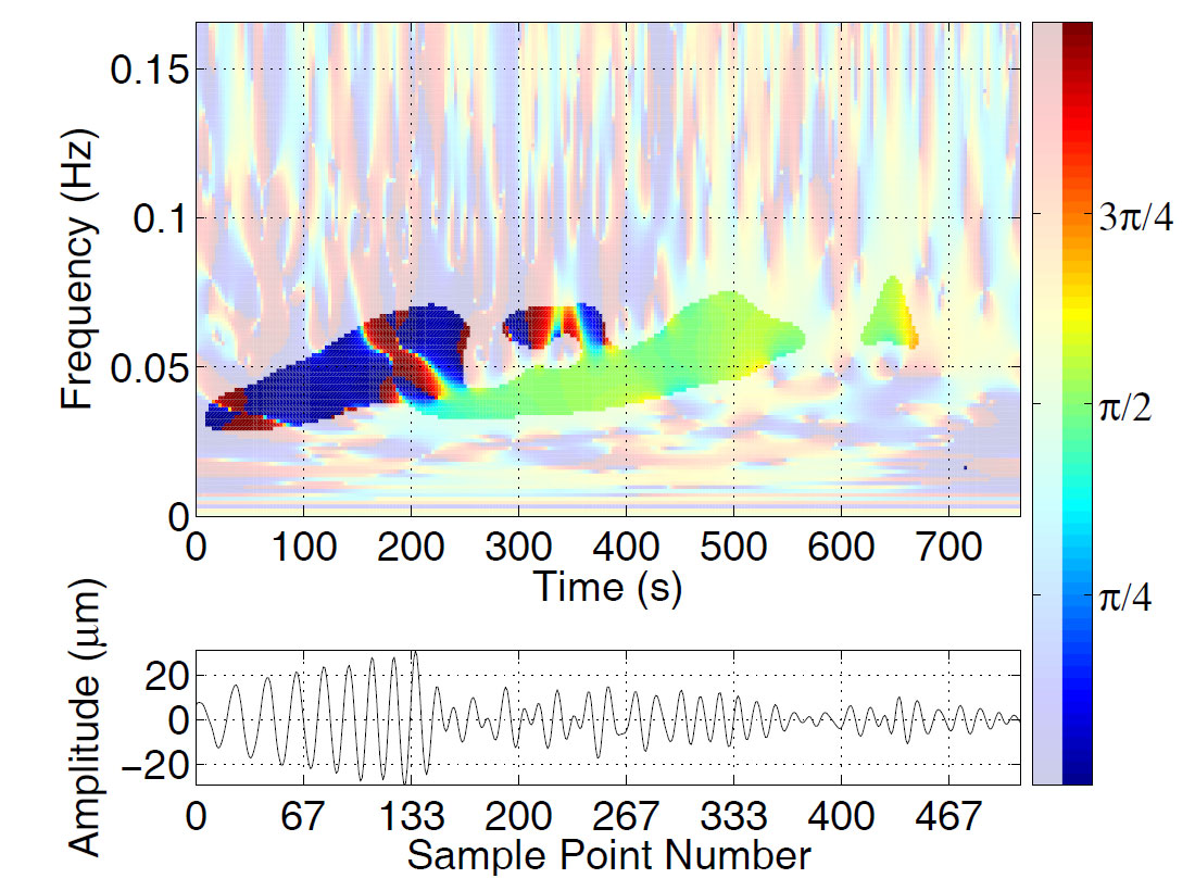
The TFR of the dip of the ellipse plane is shown in Figure 7. This spectrum is more difficult to interpret than Figures 5 and 6, because it assigns a value to the dip at every point on the time-frequency plane, regardless of whether the ellipse associated with that time and frequency makes any significant contribution to the signal. One way of addressing this problem is to use two different shades of each colour to denote dip angle, with the brighter shade being used only in regions that have large amplitudes, and the dimmer shade used everywhere else. This technique allows us to delineate the signatures of the Love and Rayleigh phases. As one would expect, the Rayleigh wave, with its vertical ellipse plane, turns out to have a dip near π/2. The wide range of dip values exhibited by the Love wave signature may seem surprising at first, since we know that Love wave motion is nearly horizontal. However, it must be kept in mind here that the dip of the ellipse plane is not the same as the plunge of the major axis of the ellipse. The ellipses that describe the Love wave are extremely elongated, and, as a result, even small noise contributions can drastically change the dip.

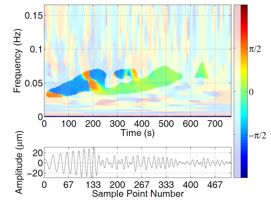
The strike TFR is shown in Figure 8. Here the behaviour of the Love phase is easier to understand. Its value is generally near ±π/2 ( relative to the positive radial direction), as one would expect for a transverse wave. The reason there are two possible values of strike that are π radians apart has to do with our definition of “strike” which has to account for the direction of particle motion around the ellipse. We define the strike to be the azimuth the particle has when it crosses the horizontal plane in an upward direction. Thus reversing the direction of particle motion changes the strike by π. (It also changes the dip from from I to π- I, turning clockwise motion into counterclockwise motion, or vice versa.)

The Rayleigh wave signature has a more stable strike with a value near 0. This tells us that the particle is displaced towards the positive radial direction when it rises through the horizontal plane, which is consistent with the known retrograde motion of the Rayleigh wave. The pitch of the major axis is shown in Figure 9 and here it is no surprise to learn that the Rayleigh wave’s pitch is almost exactly π/2 (i.e. its long axis is nearly vertical), while the Love wave, being horizontal, has a pitch that alternates between 0 and π. Since the pitch angle is measured with respect to the strike direction, a change in one usually is associated with a change in the other.

Time-frequency polarization filtering

The Stockwell TFR is invertible and can be used to design workable signal-adaptive polarization filters that target events that have specific polarization properties. There is considerable flexibility in the filter design, because we are not restricted to simply reducing the amplitude of a targeted ellipse; instead, we could also hold its shape constant while altering its dip angle, or rotate it about the vertical axis to align its strike with the direction of wave propagation. Alternatively, we could reduce its minor axis to zero, without changing its major axis. Specific times and frequencies may also be targeted. There are many possible filter types.

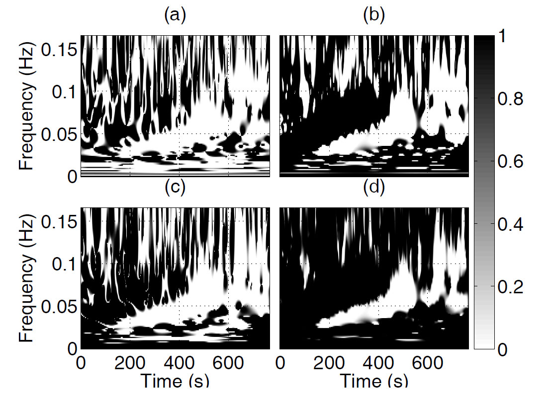
The particular filter I have applied to Figure 3 to produce Figure 10 is designed to attack the Rayleigh wave. This filter is only active in the parts of the time-frequency plane for which the dip, strike and ellipticity are all reasonably consistent with Rayleigh-type behaviour (the masking functions that determine where the filter is active are shown in Figure 11). When it is active, the filter assumes that any elliptical-type motion is due to ground roll that has a 3:2 major-to-minor axis ratio. It leaves the dip, strike and pitch of each ellipse unchanged, but reduces both the major and minor axes of the ellipse, with the reduction in the major axis always being 50% larger. The greyscale of Figure 11d gives the degree of reduction; in the “white” regions, the minor axis is reduced to zero or nearly zero. In Figure 10, we can see that nearly all of the Rayleigh-type motion has been removed.

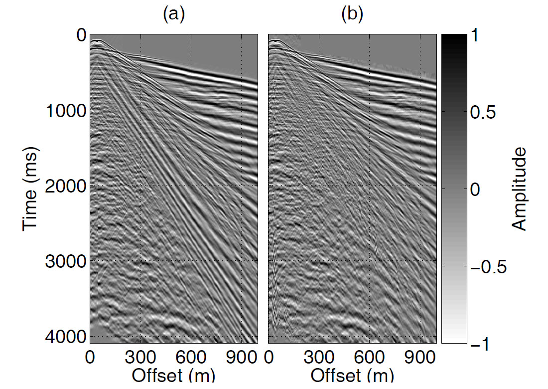
As a second example, Figure 12a shows the vertical component of a three-component shot gather, and Figure 12b shows the same shot gather after trace-by-trace adaptive filtering. For each trace the filter was designed according to the same criteria as in Figure 11. Much of the ground roll has been removed and some previously obscured signal has become visible. For presentation purposes, AGC has been applied to both Figures 12a and 12b; this was done after the filtering.

Acknowledgements

It is a pleasure to thank David W. Eaton of the University of Western Ontario for providing the seismic trace (obtained from the POLARIS seismic network). The shot gather of Figure 12 was provided by an oil and gas company that have requested anonymity; I gratefully acknowledge their contribution. I also thank Blackwell Publishing for granting permission to reproduce some of the figures from my GJI article (cited following).