The old and the new in seismic inversion

Introduction

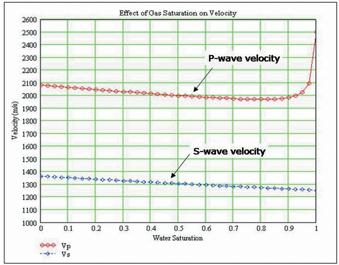
Seismic inversion is a technique that has been in use by geophysicists for over forty years. Early inversion techniques transformed the seismic data into Pimpedance (the product of density and P-wave velocity), from which we were able to make predictions about lithology and porosity. However, these predictions were somewhat ambiguous since P-impedance is sensitive to lithology, fluid and porosity effects, and it is difficult to separate the influence of each effect. To perform a less ambiguous interpretation of our inversion results, we must perform full elastic inversion, in which we estimate P-impedance, S-impedance (the product of density and S-wave velocity) and density. The reason for this can be seen in Figure 1, which plots the P and S-wave velocities as a function of gas saturation. In this figure, it can be noted that the P-wave velocity drops dramatically when gas is introduced into the reservoir whereas the S-wave velocity is largely unaffected by the introduction of the gas.

This talk will present both a history of seismic inversion and an overview of the inversion techniques themselves.

Seismic interpretation

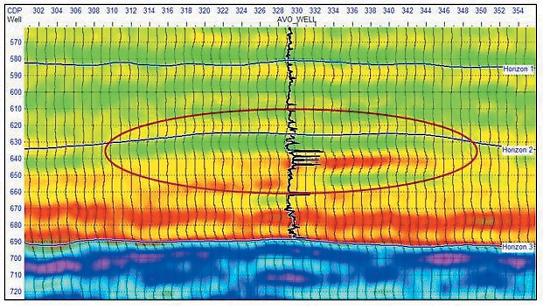
The seismic reflection method was developed in the first quarter of the twentieth century and was used initially as a tool for identifying structures, such as anticlines, which could act as trapping mechanisms for hydrocarbon reservoirs. Such a structure can be seen in Figure 2, which shows a seismic line recorded over a gas-charged sand. The high on the picked structure corresponds to the gas sand. The inserted curve is the P -wave sonic log. But this structural interpretation is ambiguous when it comes to identifying gas sands. By the 1970s, geophysicists had started to realize that information was contained in the amplitudes of the seismic reflections themselves. This information could be correlated with porosity changes, lithology changes, or even fluid changes within the subsurface of the earth.

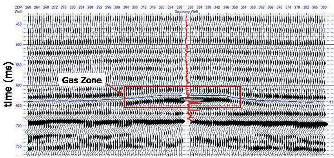
The amplitude anomalies on a seismic section became known as “bright-spots” and were considered to correlate well with gas sands. A typical “bright-spot” is highlighted by the rectangle in Figure 1, and is associated with the gas sand. Unfortunately, “bright-spots” were also ambiguous with respect to identifying fluid anomalies, which lead to the development of the AVO (amplitude variations with offset) technique, to be discussed later. However, let us first look at how we can “invert” the section shown in Figure 2.

Post-stack seismic inversion

The seismic traces in the stacked seismic section shown in Figure 2 can be modelled as the convolution of the earth’s reflectivity and a bandlimited seismic wavelet, which can be written

where s_t is the seismic trace, w_t is the seismic wavelet and r_t is the reflectivity. The reflectivity, in turn, is related to the acoustic impedance of the earth by

where r_Pi is the zero-offset P-wave reflection coefficient at the i^th interface of a stack of N layers and Z_Pi=ρiV_Pi is the ith ρ-impedance of the i^th layer, where ρ is density, V_P is P-wave velocity and * denotes convolution. Lindseth (1979) showed that if we assume that the recorded seismic signal is as given in equation (2), we can invert this equation to recover the P-impedance using the recursive equation given by

By applying equation (3) to a seismic trace we can effectively transform, or invert, the seismic reflection data to P-impedance. However, as also recognized by Lindseth, there are a number of problems with this procedure. The most severe problem is that the recorded seismic trace is not the reflectivity given in equation (2) but rather the convolutional model given in equation (1). The effect of the bandlimited wavelet is to remove the low frequency component of the reflectivity, meaning that it cannot be recovered by the recursive inversion procedure of equation (3).

After proper processing and scaling of the seismic data, an intuitive approach to recovering the low frequency component is to simply extract this component from well log data and add it back to the seismic. However, this is a fairly ad-hoc procedure, and a more recent approach to inversion is called model-based inversion (Russell and Hampson, 1991). In model-based inversion we start with a low frequency model of the P-impedance and then perturb this model until we obtain a good fit between the seismic data and a synthetic trace computed by applying equations (1) and (2). Both recursive and model-based inversion use the assumption that we have extracted a good estimate of the seismic wavelet. The extracted wavelet from the stacked section of Figure 2 is shown in Figure 3, where the time domain response of the wavelet is shown on the left, and its frequency domain response on the right.

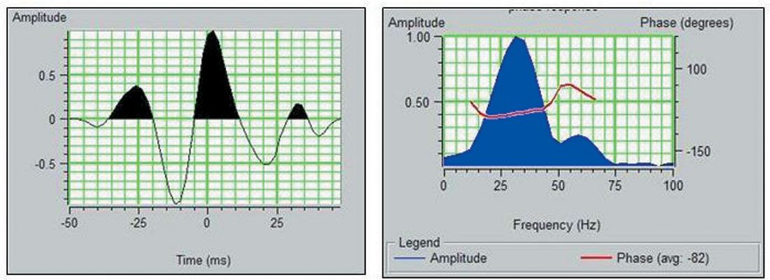
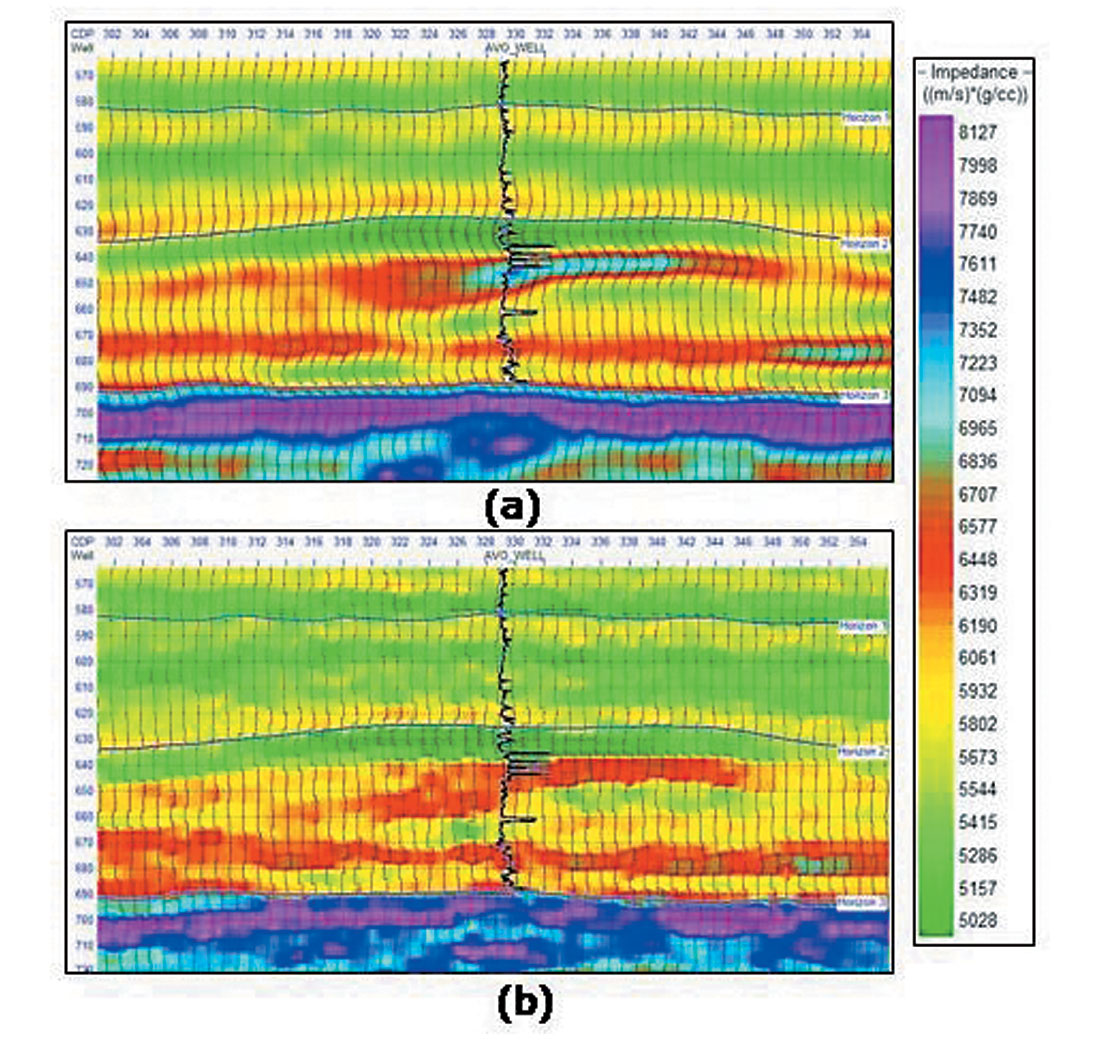
Figure 4 shows the inverted sections for the seismic line in Figure 2, where the top inversion was done using the recursive technique and the bottom inversion was done using model-based inversion. In Figure 4, notice that although the model-based results looks a little more geologically reasonable (it has a blockier, less smoothed appearance, and less dramatic swings), both inversions show a low-impedance zone at the gas sand zone, which is to be expected. However, there are also low impedance zones elsewhere on both inversions, probably due to shales. Thus, low impedance associated with “bright” amplitudes is not an unambiguous indicator of a gas sand.

Pre-stack simultaneous inversion

The standard seismic data processing flow involves transforming a set of CMP gathers into a stacked section. For example, a few of the processed gathers that were used to create the section shown in Figure 2 are shown in Figure 5, along with a “cut-out” of the stacked section within the zone corresponding to these gathers.

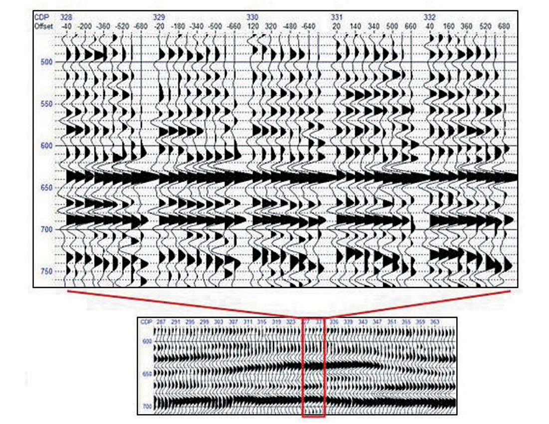
The assumption behind stacking is that the amplitudes on the gather do not show much variation, so that stacking can be considered as simply a noise cancellation technique. However, if we look carefully at the gathers in Figure 5 around the zone of interest (630 ms) it is clear that the amplitudes show a lot of variation from the near offset on the left to the far offset on the right. In this case, we see an increase in amplitude, often associated with an anomaly in which the impedance of the gas layer is less than that of the surrounding shales.

The reason behind this can be seen in Figure 6, which shows that an incident P-wave at an angle θ results in reflected and transmitted P and S-waves. This is called mode conversion, and the amplitudes of the reflected and transmitted waves can be computed using the Zoeppritz equations (Zoeppritz, 1919).

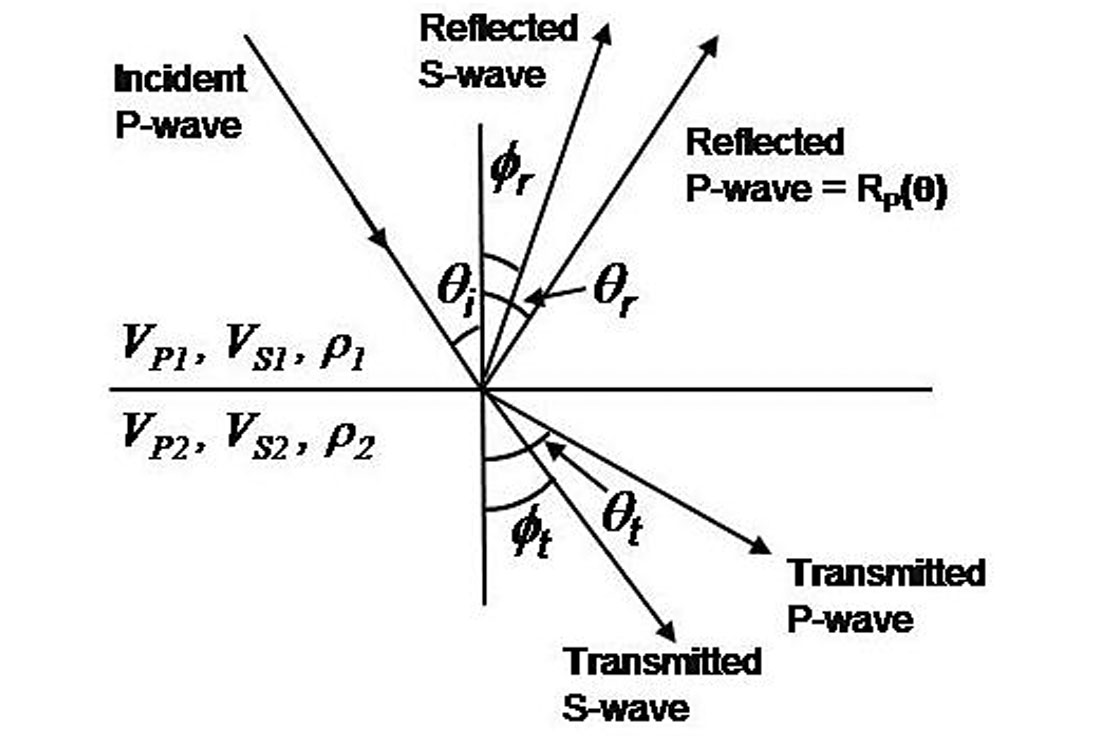
The Zoeppritz equations are a set of four equations in four unknowns that are difficult to intuitively interpret. However, as shown by Aki and Richards (2002) a linearized version of these equations can be written for the reflected P-wave in which we divide the response into three terms. In the original Aki-Richards equation, the three terms were weighted values of changes in P-wave velocity, S-wave velocity and density. However, their equation was reformulated by Wiggins et al. (1983) as

where

is a linearized approximation to the zero-offset P-wave reflection coefficient,

Equation (4) forms the basis for the AVO (amplitude variations with offset) method, in which the terms A and B, called intercept and gradient, are extracted from the seismic data using a weighted stack method and are cross-plotted and analyzed for fluid anomalies. We will not discuss AVO in this article, but rather jump directly to pre-stack inversion, which can be considered as a quantitative extension of AVO.

The Aki-Richards equation was re-formulated by Fatti et al. (1994) as a function of zero-offset P-wave reflectivity R_P0, zero- offset Swave reflectivity R_S0 and density reflectivity R_D in the form

where

and

R_P0 is equivalent to the A term in equation (4), and the other two reflectivity terms are given by

Based on equation (5), a least- squares procedure can be implemented to extract the three reflectivity terms from the pre-stack seismic data.

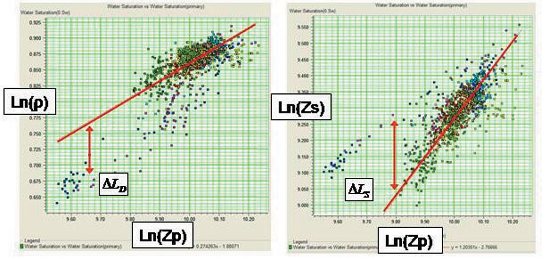
After we have extracted the three reflectivities in equation (5), they can be inverted using the post-stack inversion method described in the last section. This is referred to as independent inversion. However, Hampson et al. (2005) developed a new approach that uses a modification of equation (5) and allows us to invert directly for P-impedance, S-impedance, and density. This method is referred to as simultaneous inversion. It was also the goal of this work to extend the model-based post-stack impedance inversion method described in the last section to perform pre-stack inversion. Although the mathematics of this approach will not be described here (the interested reader is encouraged to read the expanded abstract by Hampson et al., 2005), one of the key assumptions in simultaneous inversion is that we can build linear relationships between the logarithms of P-impedance and S-impedance, L_P and L_S, and between L_P and the logarithm of the density reflectivity, L_D. That is, we are looking for deviations away from this linear fit given by ΔL_S and ΔL_D, as illustrated in Figure 7.

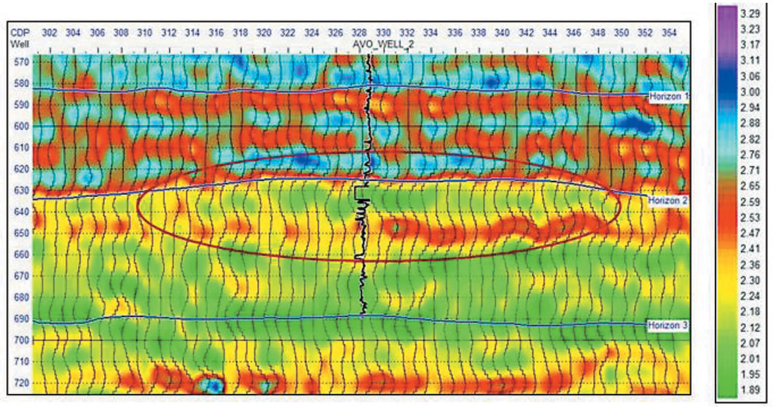
The inverted P-impedance from the simultaneous inversion of the pre-stack data in Figure 5 is shown in Figure 8, and displays less of an impedance drop than the model-based post-stack inversion shown in Figure 4. This is to be expected, since the amplitudes used in the post-stack inversion were increased due to the AVO effect. As in post-stack inversion, the P-impedance on its own is not a gas sand indicator.

However, when we combine the plot shown in Figure 8 with the ratio of the inverted P and S-impedances (which gives the V_P /V_S ratio since the density terms cancel) shown in Figure 9, the interpretation becomes more clear. Associated with a drop in P-impedance is a drop in the V_P /V_S ratio, which is generally an indicator of a gas sand.

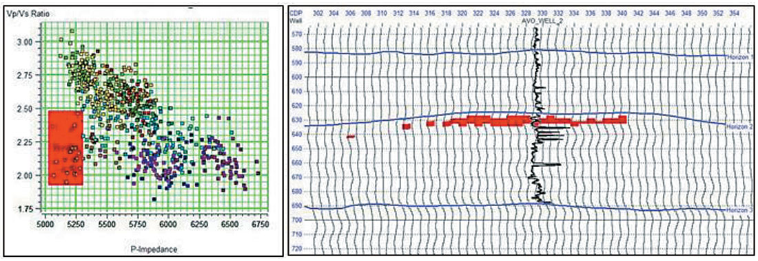
To show this more conclusively, Figure 10 show the results of a crossplot of a small portion of the two sections shown in Figures 8 and 9. On the crossplot itself, shown on the left of Figure 10, we have highlighted a zone in which both P -impedance and V_P/V_S ratio are low. This zone is displayed on the seismic section on the right-hand image in Figure 10. Notice the excellent definition of the gas sand zone.

The example we have been considering is a 2D example and the method discussed in this talk can be applied to 3D datasets to give a spatial image of the reservoir. Such an example, taken from the Gulf of Mexico, will be shown in the expanded version of this talk given during the CSEG luncheon.

Conclusions

In this talk, we have discussed the history of seismic amplitude inversion, from its origin as a post-stack process to the most recent developments which involves the simultaneous inversion of pre-stack seismic data. Although post-stack inversion is a powerful and robust method, it suffers from the fact that its final product, P-impedance, does not allow us to discriminate between lithology, porosity and fluid effects. This limitation was removed with the development of both the AVO technique and simultaneous inversion of pre-stack data. The simultaneous inversion method that we discussed is based on the assumptions that reflectivity as a function of angle can be given by the Aki-Richards equation, and that there is a linear relationship between the logarithm of P-impedance and both S-impedance and density. We illustrated our inversion methods using a gas sand example from Alberta.