The influence of HTI anisotropy on microseismic event location – a case study from a tight gas field in British Columbia

VTI anisotropy has been proven to have a large impact on the location accuracy of microseismic events associated with hydraulic fracture monitoring (e.g., Erwemi et al., 2010, Maxwell et al., 2010 ). However, the influence of HTI anisotropy on microseismic event location has rarely been taken into consideration and measured. Measurement of sensor orientation in a vertical monitoring well from perforation shots during a hydraulic fracture monitoring at a tight gas field in British Columbia in western Canada illustrated the influence of HTI anisotropy is significant on both sensor orientation and microseismic event location. Ignorance of the impact of these factors will lead to drastic lateral event location errors, distortion of microseismic imaging, and misleading interpretation. In this study, we present a method to derive HTI Thomsen’s anisotropy parameters inside the reservoir, which can be used for the reference of sensor orientation and microseismic event location calibrations. In addition, the inverted direction of axis of symmetry of HTI media provides an alternate method to estimate the direction of aligned vertical fracture direction and/or maximum horizontal stress.

Introduction

Microseismic monitoring during hydraulic fracturing has become an important method in determining the fracture geometry of induced fracture networks and stress directions in unconventional oil and gas reservoirs. Uncertainty of the calculated microseismic event locations are generally considered to depend on the accuracy of phase time picking, sensor orientation measured from the seismogram of known sources, velocity model calibration, and reservoir-array geometry (e.g., Maxwell et al, 2010, Warpinski et al., 2005). For microseismic events monitored by a downhole vertical array, the polarization, or hodogram, is a critical factor to determine the accuracy of the sensor orientation and eventually the event azimuth and location.

Polarization is the trajectory of particle motions resulting from the seismic wave propagation and depends on the medium. In isotropic- homogeneous media, the polarization for P-waves is linear in the wave propagation direction, and for S-waves is linear normal to the wave propagation direction. As polarization depends on propagation direction from the known seismic sources to geophone array, it is straight forward to find out the azimuth of the geophone orientation. However, the actual earth model is much more complex than a lateral invariant isotropic-homogeneous medium. Numerous 3D surface seismic surveys have shown that HTI anisotropy has an effect on the seismic velocities and amplitudes due to the presence of unequal horizontal stresses and/or vertical aligned fractures (e.g., Abdullatif and Watkins, 2000, Zheng and Dragana, 2004, Zhou et al., 2011). Measurements of the shear wave splitting (SWS) and source mechanisms using microseismic data on non-vertical propagating shear waves also proved the impact of HTI media on microseismic SWS, and were used as approaches to invert aligned vertical fractures (e.g., Verdon et al. 2009, Wüestefeld et al., 2010, Rutledge and Phillips, 2003). In this study, we identified the evidence that HTI anisotropy influences the determination of sensor orientation due to the difference between the group and phase angles of the ray path and hence distorts the microseismic event location. As the velocities of both compressional and shear waves vary with the incidence angle to the symmetric axis of the HTI anisotropy medium, it is obvious that the offsets of microseismic event location will be impacted as well by its existence.

Similar to VTI, HTI anisotropy can be quantified by estimating the three Thomsen’s parameters epsilon (ε), delta (δ), and gamma (γ) (Thomsen, 1986). By measuring the difference between group and phase angles of ray paths from known seismic sources to receiver array, HTI anisotropic parameters were inverted through fitting the theoretical curves calculated on a HTI model assumption. The symmetric axis of HTI, which is generally perpendicular to the aligned vertical fracture direction and/or the maximum horizontal stress, could also be inverted through this process. At last, a workflow to determine the influence of HTI anisotropy on microseismic event location is proposed. It should be stressed that due to the complexity of natural fracture networks, application of this method may not be adequate to all unconventional microseismic monitoring.

Data and processing

Data acquisition

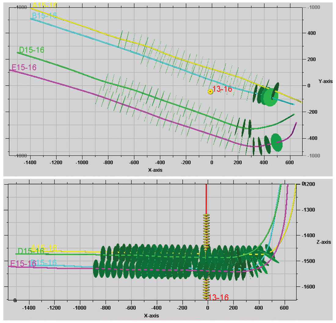
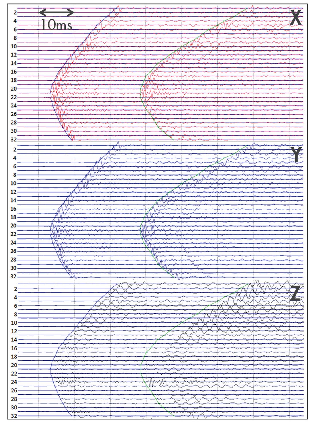
Microseismic monitoring was carried out in the a tight gas reservoir in British Columbia, by deploying a 32-level 3C geophone array in the vertical 13-16 observation well to monitor the horizontal treatment wells (A15-16, B15-16, D15-16, and E15-16) (Figure 1). The geophone arrays were clamped to the casing of the wellbore during the observation of perforation shots in the treatment wells and the hydraulic fracturing monitoring activities. Geophones in the vertical array were generally well clamped and provided good quality seismic waveforms for polarization analysis of sensor orientation process, except for two slightly weak levels at geophone #4 and #19 (Figure 2). Continuous microseismic data were recorded with a sampling rate of 0.25 milliseconds. The geophones were not moved until the end of the entire monitoring.

Sensor orientation

Typically, the sensor orientation for the downhole geophone array in a vertical monitoring well is carried out by assuming an isotropic-homogenous medium. Good-quality perforation shots in the adjacent treatment wells were selected as known seismic sources to determine the orientation of each geophone. A total of 97 good S/N perforation shots in the adjacent four treatment wells, A15-16, B15-16, D15-16, and E15-16, were used for the process (Figure 1 and Figure 2).

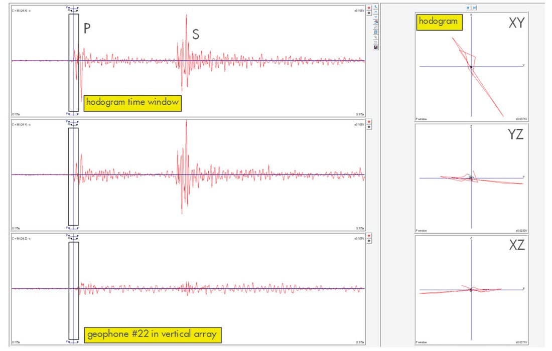
To obtain stable estimates of polarization angles, a time window covering approximately a full period from the P-wave first arrival of each waveform was used for the analysis (Figure 3). Polarizations with the linearity over 70% in the horizontal components X and Y were selected for final determination. Sensor orientation is considered to be a straight forward process based on the assumption of a lateral isotropic homogenous model, where the P-wave particle motion is considered in the direction of the propagation of the straight line ray path, and thus points back to the source (Warpinski, 2009).

Theoretically, the final azimuth of the sensor orientation of each geophone in a true vertical array should be independent to the perforation positions although slight perturbations among shots may exist due to background noise and heterogeneity along the propagation of ray paths. This type of error generally shows the features of a random pattern in the distribution among shots.

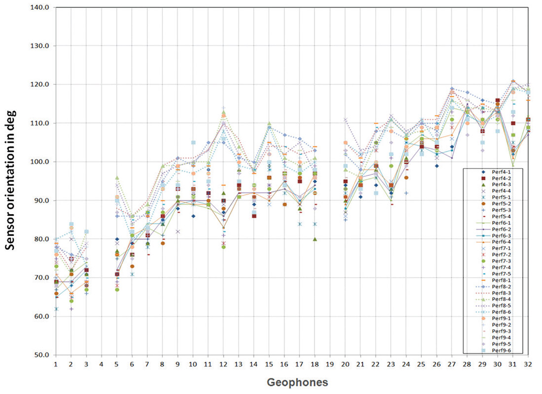
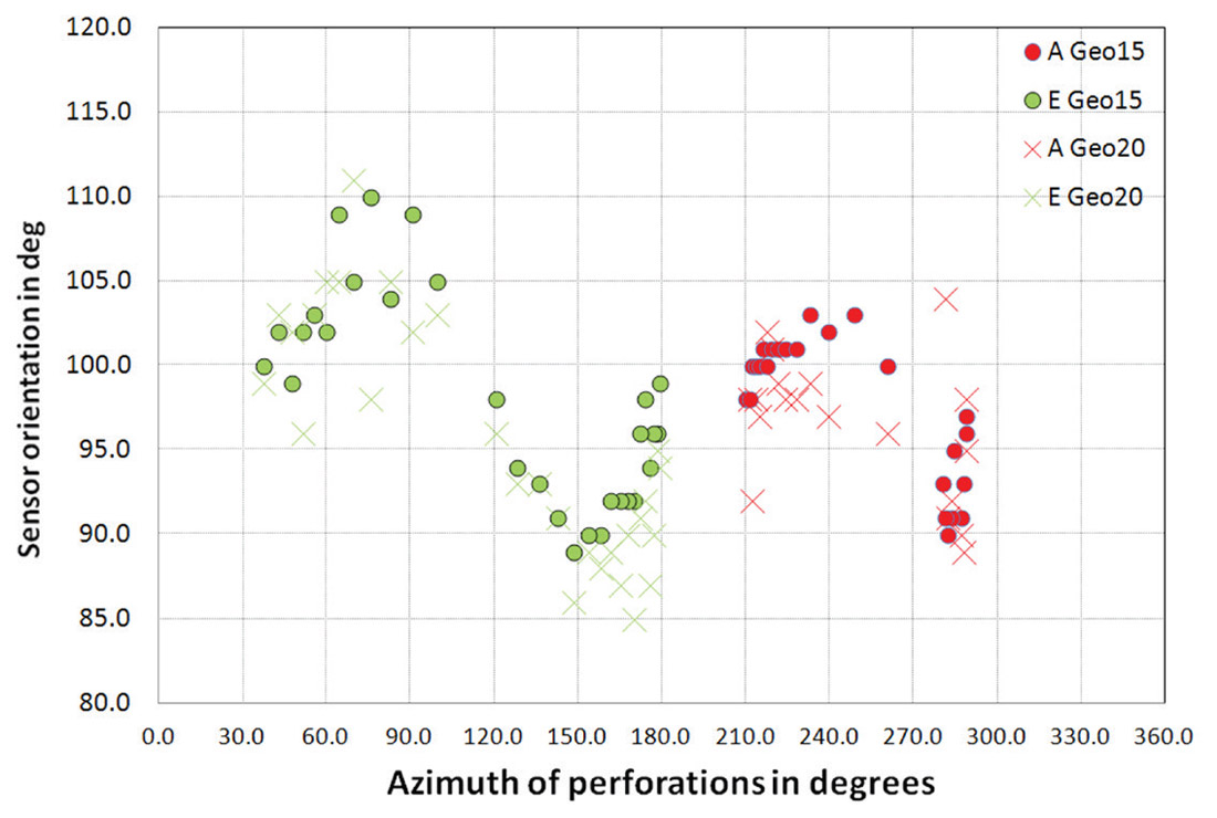
Figure 4 illustrates the measured results of sensor orientation of the geophones in the vertical array from the perforation shots fired from the closest stages in the E15-16 well. It is easy to notice the scatter in these measurements ranging from approximately +/- 10 degrees in the orientation of geophones. Measurements from other A15-16, B15-16 and D15-16 wells show a similar scattering pattern and ranges of magnitude. A scrutiny of the error distribution reveals the scattering pattern is in a systematic distribution among shots rather than a random one. This observation is quite different from the random pattern which would be consistent with the general assumption of isotropy along the ray paths of propagation.

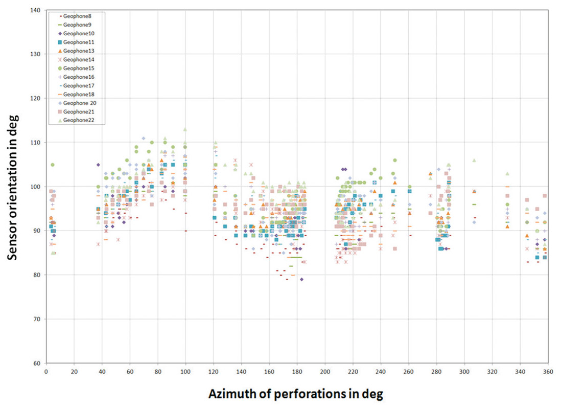
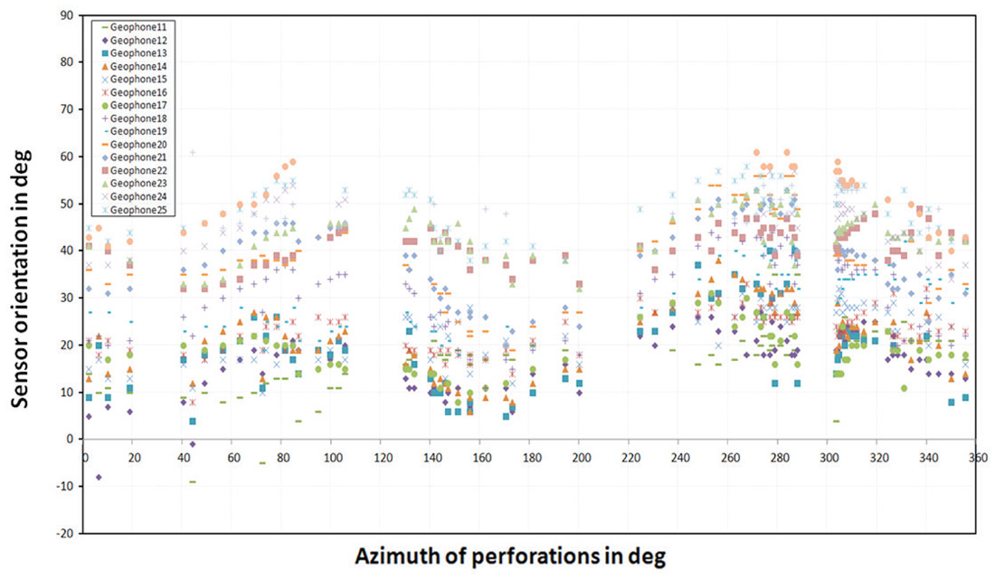
In order to examine the systematic variations of sensor orientation among the perforation shots quantitatively, error versus shot-array azimuth of the perforations were plotted from geophone levels #8 to #22, which were positioned from top to bottom in the reservoir (Figure 5). Statistically, variation of orientation of geophones shows two obvious periods of coherence within 360° of azimuth. Magnitudes of the variations from a peak to a neighboring trough generally fall in a range of 20°-25°. Two peaks of variations appeared at about 100° and 280°, and two troughs rest at 170° and 350° in azimuth. In addition, analysis of a neighboring similar microseismic project in the reservoir shows more typical characteristics than this data set (Figure 6).

HTI anisotropy correlation

Regarding the causes of such a phenomenon, three potential possible factors can be considered: well-coupling drift of the sensors due to residual torque in the wireline, dipping structural variation and transverse isotropy with a horizontal axis of symmetry medium (HTI anisotropy).

Sensor orientation of the geophones from the perforations shot at the beginning and end of the monitoring period were compared, and no noticeable time-variant drift was identified (Figure 7). Dipping structural variation might introduce cyclic orientation variation due to dip of formations, however, the main horizons from 3D surface seismic and well logs shows flat to gentle dips less than 1.5 degrees in the study area. Thus it is unlikely to influence the sensor orientation to such a large magnitude range and lead to a systematic error distribution. The last possible factor, HTI anisotropy, is an effective azimuthal anisotropic model to describe the condition of vertical aligned parallel fractures in isotropy medium (e.g., Dong, et al., 2000, Rutledge and Phillips, 2003, Verdon et al., 2009, Wüestefeld et al., 2010). Based on the microseismic imaging, core analysis, and geomechanical information in the tight gas reservoir, the direction of dominant vertical fractures and maximum horizontal stress is approximately appointing to NE40°.

An HTI anisotropy medium can be derived from a VTI anisotropy medium by transposing the vertical symmetrical axis into a horizontal one for the angle and velocity equations between group and phase seismic waves. To quantity the effects of HTI anisotropy on angle and velocity changes, the general practice in seismic industry is to use the “weak anisotropy” approximation given by Thomsen (1986). Based on Thomsen’s approximation, the relationships between group angle and phase angle for quasi-compressional and quasi-shear waves are listed below (Eqs.1-2),

Where ϕ is the group angle between source-array direction and axis of symmetry in a HTI medium; ϑ ; is the measured phase angle; ε, δ and γ are the Thomsen’s parameters for quasi-compressional and quasi-shear waves.

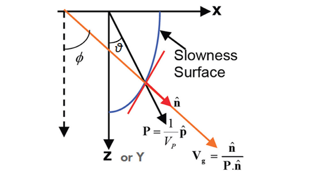
The influence of HTI parameters ε, δ and γ on the measurement of direction of ray path is well illustrated in Figure 8 by Mallick (2008). For more details, the difference between group and phase angles for a quasi-compressional wave induced by the combination of ε, δ parameters are calculated and plotted together in Figure 9. Similar calculation for a SH quasi-shear wave caused by γ are illustrated in Figure 10.

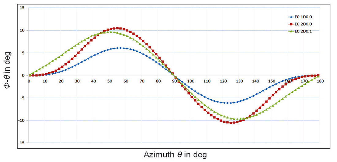
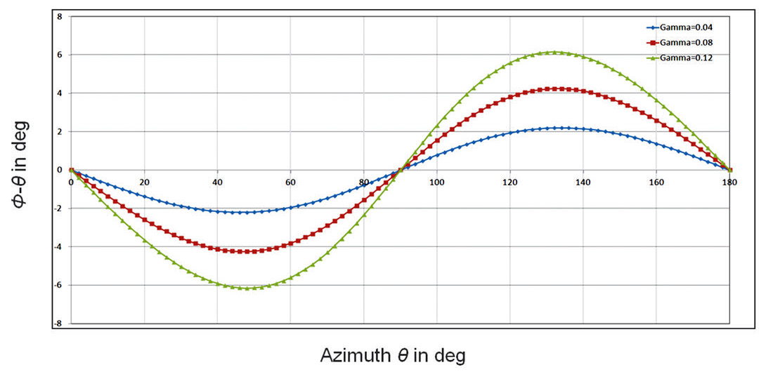
From these calculations, it is obvious that weak ε, δ and γ anisotropic parameters can induce considerable angle differences even though in a weak HTI anisotropic medium. Angle difference between group and phase angles turn to diminish when the incidence angle of ray path is parallel or perpendicular to the axis of symmetry. This observation is useful for the selection of seismic sources for an accurate sensor orientation without bringing the angular errors into the final determination.

The influence of HTI anisotropy on quasi-compressional and quasi-SH wave velocities, are also given by Thomsen (1986) in Eq.3-4. These equations will be used for the further analysis of the effect of a HTI medium on the microseismic event location afterwards.

Where V_P0 and V_SH0 represent the propagation velocities along axis of symmetry or the slow direction; the other symbols are the same as described in Eq.1-2.

To measure the magnitude and phase shift of the observed angle difference curve from sensor orientation process for the quasicompressional first arrivals of the perforations, a HTI anisotropic model with the parameters ε and δ were used to accomplish the best fitting process by a least-square method. Similar effort was carried out for the quasi-shear first arrivals with less available data despite of the natures of poor shear hodograms. For each geophone, the average of the measured sensor orientation was removed in order to obtain the net variation before starting the best fitting.

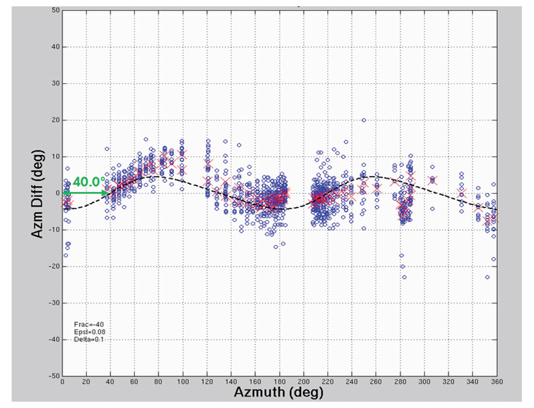
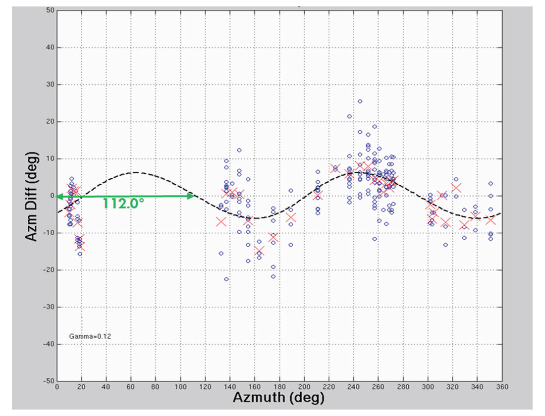
As a result, the best fitted parameters ε and δ are 0.08 and 0.10 respectively, and an azimuthal phase shift of 40.0° was derived from the quasi-compressional first arrivals (Figure 11). The measured anisotropic parameters ε and δ are relatively moderate and fell into the range similar to the VTI measured in the previous work in the areas. It is worth to stress the meaning of the measured azimuthal phase shift of 40.0°, is consistent to the results from microseismic imaging and maximum horizontal stress. Obviously, this technique provides an alternate applicable method to invert such directions in an unknown area. On the other hand, a best fitted parameter γ is derived from the 38 available quasi-shear arrivals (Figure 12). The phase shift of 112.0° derived from the less reliable quasi-shear arrivals indicates that the particle motion of the quasi-shear waves is basically perpendicular to the quasi-compressional waves.

Offset calibration

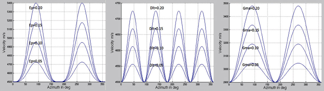
As mentioned earlier, aside from the azimuthal influence on the sensor orientation of the geophones, the existence of a HTI anisotropy medium also affects the compressional and shear wave velocities, and hence, the positioning of microseismic events. Figure 13 below illustrates some results from numerical experiments and shows the impact of Thomsen’s anisotropy parameters on the velocities of compressional and shear waves.

To quantify the influence of HTI media on the microseismic event position, an isotropichomogeneous medium near the reservoir level is assumed for simplicity of calculation. The basic equation used for the calculation of offset is simply as Eq. 5,

where D_i is the offset from a microseismic event to the i^th geophone, V_p is the compressional velocity, V_s is the shear velocity, T_pi is the time of the P arrival for the i^th geophone, T_si is the time of the S arrival for the i^th geophone, and T₀ is the time of original of the event.

Eq. 6 states that the offset D_i from an event to the i^th geophone is proportional to the time difference between the shear and compressional arrivals, T_si – T_pi. In a HTI medium, however, V_p and V_s are related to the incidence angle ϑ, and should be replaced by Eq. 3 and 4. As a result, the offset after calibration can be expressed in Eq. 7 as,

Microseismic event location calibrations and workflow

Based on the previous analysis of the influence of a HTI medium on the determination of sensor orientation and the offset and azimuth of microseismic events, we believe two types of calibrations need to be considered in the microseismic event location process in future workflows.

Different from the existing workflow used in the microseismic industry, initial information on a HTI medium in the monitoring area is necessary for the sensor orientation. When carrying out sensor orientation, appropriate seismic source locations should be selected by considering their azimuthal relationship to the monitoring array and axis of symmetry of a HTI medium. In case of already completed microseismic monitoring projects, or those projects without ideal source-array geometry, calibration of sensor orientation should be redone using the equations associated with the angular difference provided in this study.

The second difference is that the existing workflow assumes an isotropic medium for the microseismic event location, which often leads to mislocation in case of HTI media. Therefore, after acquiring a reliable a sensor orientation, both azimuthal and offset calibrations should be applied in order to remove these errors.

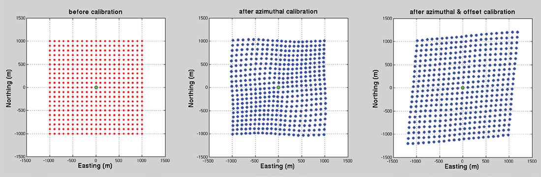
A numerical experiment was carried out to further illustrate the distortion of microseismic imaging quantitatively when the influence of the HTI anisotropy in the reservoir is ignored. Figure 14 shows the comparison of the image of locations before and after the calibrations by using the HTI parameters obtained from the tight gas field, where the direction of aligned vertical fractures/ maximum horizontal stress is assumed in NE40°, anisotropic parameters ε, δ and γ are 0.08 and 0.10 and 0.12 respectively. As a real example, angular and offset calibrations are applied to the microseismic imaging located in the study area with same anisotropic parameters as the numerical experiment (Figure 15). Clearly, the existence of HTI anisotropy has considerable influence on microseismic event location. This observation illustrates the importance of the HTI anisotropic calibrations for reliable microseismic location and further interpretations.

Conclusions

This work highlights the problems that occur in the current workflow of microseismic event location in the presence of a HTI anisotropic medium. It is clear that HTI anisotropy has a significant influence on sensor orientation and microseismic event location as well.

Through the analysis of variation of sensor orientation from perforation shots around a vertical monitoring array, HTI anisotropy Thomsen’s parameters, ε, δ and γ, can be derived by fitting the angular variation through a HTI anisotropy model.

Azimuthal phase shifts of the angular variation of sensor orientation can be used as an alternate method to invert the direction of vertical aligned fractures and/or maximum horizontal stress in an unknown reservoir.

Regarding the workflow for future microseismic data processing, two additional steps are considered:

1. Input of HTI anisotropy information prior to sensor orientation or calibration of the sensor orientation using the HTI parameters.
2. In case of HTI anisotropy, azimuthal and offset calibrations are necessary for accurate location of the microseismic events.