The impact of interbed multiples on the inversion and interpretation of pre-stack data

Unconventional resource plays commonly use a geophysical workflow involving analysis beyond stacked images and structural interpretation. This involves pre-stack quantitative interpretation methods such as inversion to obtain P-impedance and S-impedance (Z_p and Z_s) volumes that are then interpreted using rock physics and geomechanical templates (Close et al. 2012). The goal is to tease out subtle elastic properties such as Poisson’s Ratio and Young’s Modulus or mineralogical variations in order to identify sweet spots and locate spatial variations in “fracability”. Pre-stack inversion begins with seismic data which has visible coherent or incoherent noise. After inverting the data, no evidence of the removed noise remains and the interpretation continues, leading to the assumption that the inversion process has accurately removed the noise in the data. What follows is an example of how one of the coherent noise sources, multiples, can impact the inverted results and bias the interpretation.

A problem often encountered in pre-stack inversion is that the signal is contaminated with noise. This may have significant impact on inversion results and their interpretations. It is shown that small variations in distance between the primary and multiple generators can alter where the constructive/destructive interference occurs. This variation biases the inversion output, resulting in an overestimate or underestimate of Z_p and Z_s.

There are numerous techniques available to attenuate coherent noise in the prestack domain. However, quantifying how damaging multiples are to the amplitude versus offset (AVO) response is seldom addressed. The modeling approach described in this article can be used to help determine the degree of interpretation error resulting from un-attenuated multiples. It is noted that uplift may be obtained by increasing the range of angles used in the pre-stack inversion.

Introduction

common challenge in seismic processing is the identification and attenuation of seismic multiples, particularly when their residual moveout is small making them kinematically similar to that of the primary reflections. Currently, numerous methods are applied in the pre-stack domain to reduce multiple interference and enhance the stack and AVO response of the primary reflection. The most common is the Parabolic Radon Transform which relies on residual moveout of the multiple relative to a primary. There are also more advanced techniques using wave equation prediction (Jakubowicz, 1998).

The following model based approach quantifies the error in AVO interpretation of data due to multiple contamination by looking at the results of pre-stack inversion. Because of large subsurface impedance contrasts at depth produce seismic multiples with sufficient energy to return to the surface, these multiples can interfere with the primary reflection representative of the zone of interest (ZOI). Once the error in the AVO interpretation is quantified through the modelling proposed, the interpretation of pre-stack inversion attributes can continue.

Method

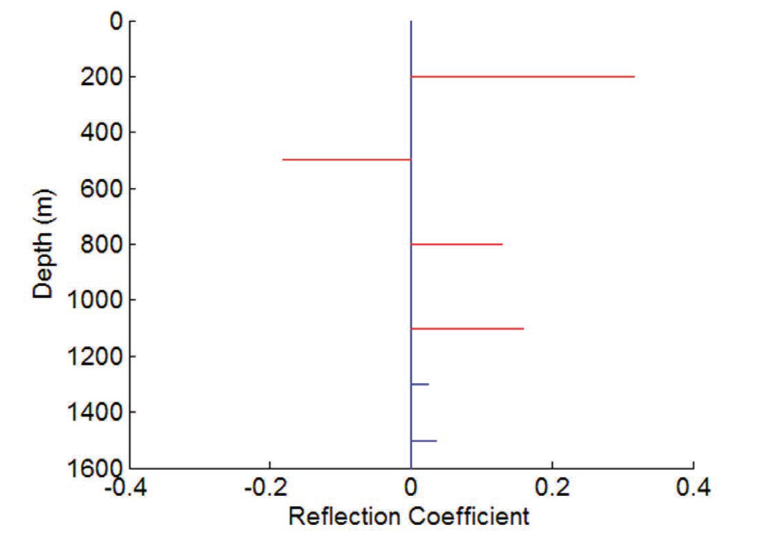
The method used to create a synthetic shot record assumes a linear elastic isotropic medium. Within this medium, 1D ray tracing is used to determine the travel path and angles of incidence at reflection points which are inputs to the Zoeppritz equations used to calculate the AVO response. The 1D domain was chosen for its ease of use and simplicity since accounting for structural components and travel path variations would only add unnecessary complexity to an approach where there are sufficient variables that can be altered and still allow for meaningful conclusions. The Zoeppritz equations were chosen over an approximation for the forward modeling of amplitudes because of their accuracy. For the primary reflections a small angle approximation would suffice. However, in the case of multiples traveling through the medium and reflecting at various incident angles off of multiple boundaries, the slight deviations from the full solution due to an approximation will compound the inaccuracy of the multiples AVO. The modelling methodology uses a layered block model, where only first order multiples are considered. The parameters for the model can be found in Table 1. The zero offset reflection coefficients are displayed in Figure 1.

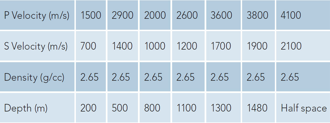
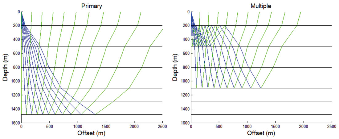
The values chosen approximate what could be expected of multiple contaminations for an unconventional reservoir. There are few strong impedance contrasts at relatively shallow depths which will generate multiples and smaller impedance variations at greater depths representing the unconventional resource. Displayed in Figure 2 are the primary reflection to be analyzed and the multiple that is contaminating the primary. It also shows the rays with angles from 0 to 20 degrees.

It is noted that a downgoing peg leg multiple (where the peg leg occurs on the downgoing ray) will have an identical response both in moveout and amplitude to the upgoing peg leg (where the peg leg occurs on the upgoing ray). This doubles the amplitude response at that given time and offset in the shot record though the response is from two separate travel paths. This may explain how certain large amplitude multiples are able to be recorded on the surface. A majority of reflectors do not have the contrast required to generate a multiple to surface after it has reflected off multiple interfaces (hence the RC cutoff of 0.1 used for modelling purposes).

Another learning from modelling is that seismic multiples have highly complicated amplitude versus angle (AVA) response. In contrast to a single ray (ray parameter p) for a primary reflection which has a single angle of incidence, when tracking a single ray of the multiple, the angle of incidence may vary for each boundary and thus the amplitude response at a given offset is a function of potentially three different incidence angles. Therefore mapping a multiple into AVA space is no simple procedure. The AVA response of a multiple will be a function of its location in time relative to the primaries used in the offset to angle calculation. This displays the necessity for modelling the seismic response in an offset domain and then transforming to angle domain to perform AVA work.

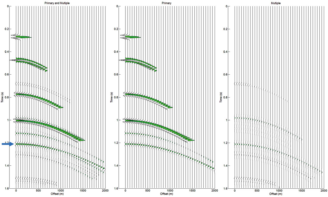
Displayed in Figure 3 is the shot record using a 30Hz Ricker wavelet. Both the primary of interest (6th reflection) and the contaminating multiple are shown in Figure 2. At this reflection, multiples appear to be contaminating the near offsets. To confirm this, the data is sorted into a common depth point (CDP) gather to preform velocity analysis and moveout correction (Figure 4). Since the velocities are known the offset to angle calculation is computed accurately. Next the amplitude is extracted on the reflection of interest (peak/ trough) to analyze the effect of multiple interference on the primary. The analysis of multiple contamination on the AVO response will be restricted to a single interface. Any errors in the estimation of P-impedance and S-impedance for a given layer could cascade to lower layers and impact estimates which are multiple free. However, the aim of this investigation is to determine the multiples influence on inversion and not how the error could propagate through inversion to subsequent interfaces in the shot record.

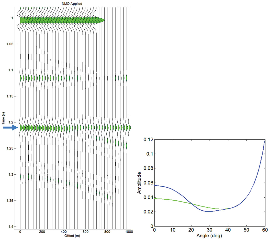
Figure 4 shows that the resulting multiples in the gather have significant residual moveout relative to the flattened primary with most contamination occurring at near angles. To quantify the error and how it will affect the interpretation of the data, the contaminated primary is inverted using the Fatti et al. (1994) approximation (Equation 1) minimizing the RMS error between the inverted result and the data shown in equation 2

where

and

are the zero offset P and S reflectivity respectively,

is the average Vs over average Vp for the two layers and

is the density difference over the average density for the two layers. For the inversion, the layer above is assumed to be known and only the P-impedance and S-impedance of the layer below are inverted for. These assumptions were used to minimize any error associated with the inversion process and to better isolate the effect of the multiples alone. The inverted results will be displayed in LambdaMuRho (LMR) space (Goodway, 2001). A brief review of the LMR templates used can be found in the appendix.

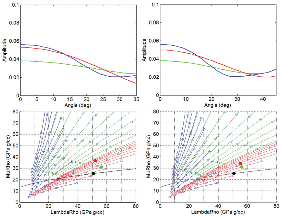
Displayed in Figure 5 is the model of Figure 4, using data out to 35 and then 45 degrees respectively to represent variations in acquisition parameters and the impact on inversion. From the inverted result several key observations can be made. First, large errors in shear impedance estimation exist even though multiple contamination was mostly restricted to near to mid angles. Second, the error in P impedance increases (the zero degree amplitude) as the angles used in the inversion decreases. Third, when offsets are sufficiently large, the inversion procedure is able to see through the coherent noise and correctly invert the primary. For both angle ranges, the inversion predicts higher Z_p and higher Z_s, or higher Young’s modulus and lower Poisson’s ratio. From a mineralogical perspective, using the limestone-clay trend the inversion places both inversion angle ranges in more porous limestone rich region of LMR space. For the 45 degree angle range there is 15% overestimate of limestone and in the 35 degree angle range nearly a 45% overestimate of limestone. The black line is the so called zero gradient line (Perez, 2010). It is defined by combination of overlying layer and underlying layer properties that together would result in no gradient. The distance of the underlying layer from the zero gradient line is proportional to the gradient.

The next model takes the same parameters as used previously but increases the multiple to primary distance by 25m. This increased distance results in the multiple encountering the primary in the mid to far offset range. In this scenario the majority of the primary AVO response is relatively noise free and only a small angle range has been degraded (Figure 6).

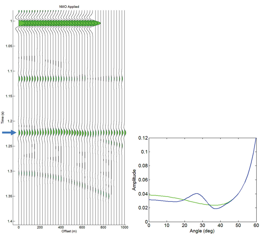
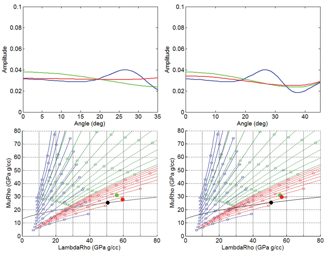
Figure 7 shows the second model, using data out to 35 and 45 degrees. The inverted result predicts a decreased Zp and Zs and an error that has a significantly different bias when compared to the previous model. For the second model a mineralogical template would predict higher clay content and a decrease in porosity. For the 45 degree angle range there is 5% overestimate of clay and in the 35 degree angle range a 10% overestimate of clay. When there is sufficient offset/ angle information and noise free data on either side of the multiple interference, the inversion essentially removes the effect of the multiple contamination.

Overall the inversion procedure does a reasonable job of estimating the correct impedances. The increased angle improves the ability of the method to see through the multiple. This stems from the Fatti equation used for inversion as it only accounts for primaries and treats all other data as noise. Multiples have two factors that this equation does not model. First the multiples are not flat in time and thus the AVA extraction will extract amplitudes at various positions of the wavelet. Secondly, assuming the multiple is flat the AVA response cannot be modeled directly by the Fatti equation because its AVA response is the combination of three separate AVA responses (first order multiple).

For both previous examples, with an increase in angle range used to invert the data there is a significant improvement in the accuracy of the inverted result. The impact of the error varies significantly depending on where the noise cuts across the primary. For the first model, when the particular peg leg multiple was concentrated in the near angles of the primary, the impact lead to increased impedance estimation error relative to the model where the multiple cuts through the mid to far angle range.

Conclusions

Two different models were shown to estimate the impact of multiples on AVO Inversion. From the two models it is shown that subtle variations in depth can have a substantial impact on the resulting inversion due to the offset range at which the multiple interferes (near/far). The impact of multiples on the result of the inversion negatively affected the interpretation of the models. The results of the inversion show that when isolating subtle variations in rock properties, coherent noise can negatively affect the inversion result and bias the interpretation. In both cases, an increase in offset increases the accuracy of the inversion.

Appendix

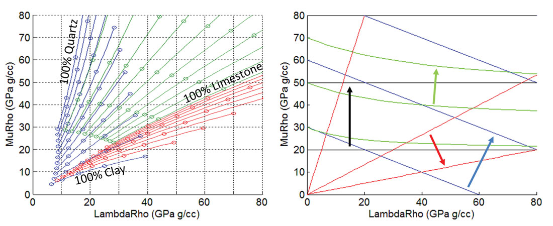
The first template in Figure App 1 shows three sets of dual mineral trends created using a non-interacting model (Perez, 2013). The three trends displayed are the quartz-clay in blue, quartz-limestone in green and limestone-clay in red. The model assumes spherical pores and no cracks where the trend lines that share a common colour are 10% increments of the noted two mineral mix. The circles along the trend lines display 10% porosity increments increasing towards the origin. Further detail on the models can be found in Perez (2013). The second template displays lines of constant Young’s Modulus, Poisson’s ratio, P-impedance and S-impedance in LMR space.

Acknowledgements

The author would like to thank Marco Perez and Christa Burry for their contributions and reviews of the article