The bleeding edge of seismic imaging, 2003

Introduction

Earlier this year, James Sun and I gave a CSEG Luncheon presentation describing the current state of the art of seismic depth migration, as it applies to Canadian basins. Our overview was aimed at bridging the gap between depth migration and velocity analysis methods routinely applied today, and newer methods that promise higher-fidelity imaging solutions for more elusive structural targets. The current methods are Kirchhoff depth migration and ray-based traveltime tomography to estimate both near-surface and deeper velocity structure. We referred to these as “workhorses”, with the implication that we should consider putting them out to pasture. The day for doing that hasn’t yet arrived, and it won’t for a while, as I will emphasize later on in this article. But several months after our presentation, we’ve seen an enormous increase in the use of new, higher-fidelity imaging methods, especially in difficult marine environments such as the Deepwater Gulf of Mexico, and we’ve even seen some startling improvements in our Foothills images using these new methods. The purpose of this article is to focus on the new imaging methods (not velocity analysis methods, which are a bit further in the future).

The new methods are not without their problems, however. Most of them, which go collectively by the name “wave-equation migration” (WEM), have problems with anisotropy, especially the tilted transverse isotropy commonly assumed in the Foothills. Most of them have serious problems with 3-D land data, which are too sparsely sampled on the recording surface to provide an adequate wavefield for the all-important downward continuation step. One of the newer methods can overcome most of these problems. It is “beam migration,” a hybrid that combines aspects of Kirchhoff migration and WEM.

The current state of the art

Kirchhoff depth migration, a new tool in the late 1980s, is familiar by now to many, if not most, structural interpreters and processors. It is versatile, allowing the migration of any selection of input traces onto any desired output grid. It honours topographic variations along the recording surface very easily, and it honours exact source and receiver locations. Its traveltime solvers have been modified to handle anisotropy (specifically TTI, transverse isotropy with a tilted symmetry axis). It is reasonably efficient. It provides migrated CDP gathers in 3-D that are used by tomography programs that estimate velocity. Figure 1 shows “typical” Foothills structural images obtained by Kirchhoff migration, both with and without the use of TTI.

The bleeding edge of imaging

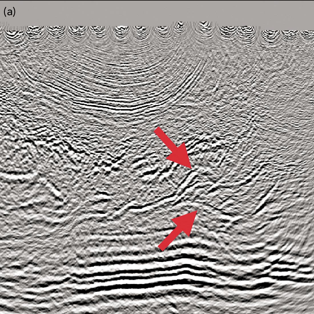
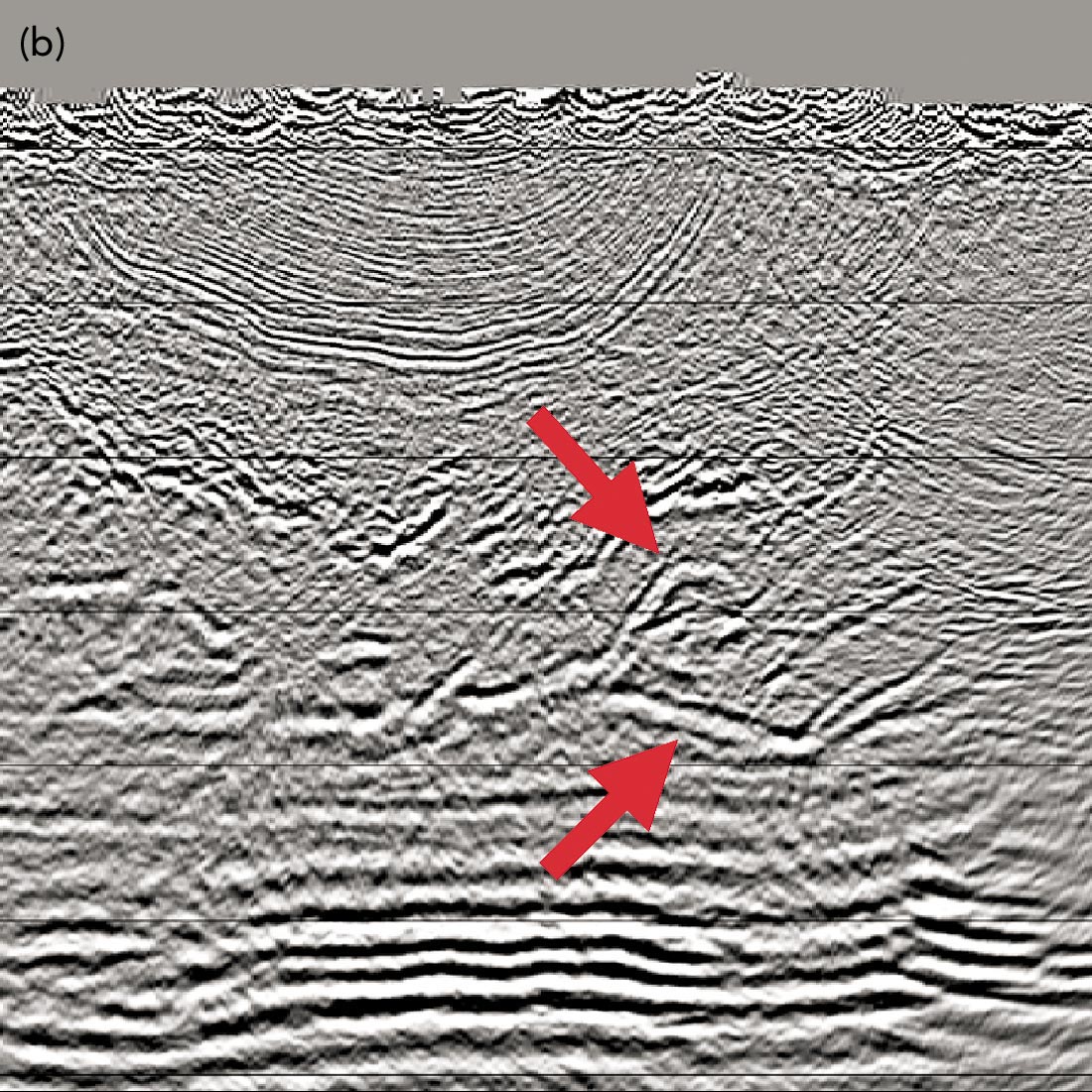
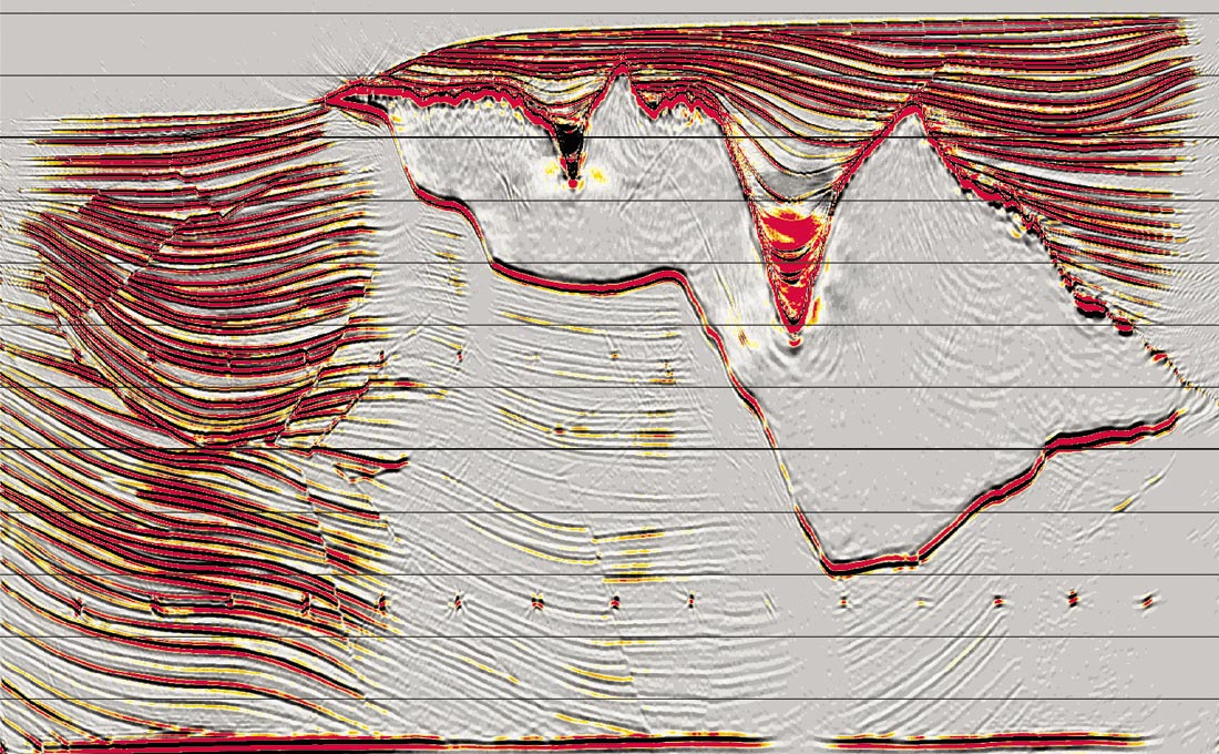
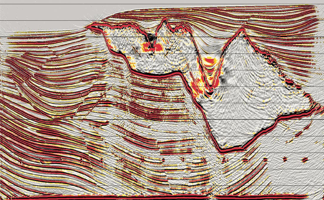
In contrast to Figure 1, Figure 2 shows “typical” Foothills images obtained by (isotropic) Kirchhoff migration and WEM. The WEM image shows clear improvement over the Kirchhoff image, especially in the reduction of migration smiles. We see differences like this to some degree on most of our Kirchhoff/WEM imaging comparisons. Often, the improvement delivered by WEM has no effect on the geologic interpretation of the image, and doesn’t warrant the extra computational effort of the WEM. In many cases, though, either noise reduction or structural improvement of the newer methods justifies their added cost.

Wave-equation migration is not new, but its routine application to 3-D unstacked data has become possible only recently as greater computing power has become available. There are many WEM methods: implicit and explicit finite-difference, Li-corrected finite-difference, Fourier finite-difference, “screen” methods such as split-step, and others, each with its special features and advantages. Most of these are based on one-way versions of the wave equation; as a result, they tend to lose the ability to image very steep dips with great accuracy. A method based on the full two-way wave equation, reverse-time migration, has no trouble imaging dips even beyond 90 degrees, but it tends to become very expensive as it images higher-frequency data.

Another family of migration methods goes by the name “beam migration” (Gaussian beam, coherent states, beamlet migration). Some of these are based on the (one-way) wave equation, while others use rays. They all operate on a part of a wavefield that is localized in both space and direction. For example, Gaussian beam migration decomposes reflection data into localized plane-wave components, then sends those components into the Earth along trajectories surrounding raypaths.

All of these methods tend to be cleaner than Kirchhoff migration. Why? Because there are so many methods, there are many reasons, but two stand out. First, most of the newer methods perform more “work” than Kirchhoff migration; they add more numbers together to get the final image. All that extra work tends to cancel noise, both random noise and the coherent swings that can bedevil a Kirchhoff image. Second, all the newer methods possess some form of implicit or explicit operator tapering, often in several different ways. For example, finite-difference methods based on the one-way wave equation have migration operators that “disperse” very gradually, and eventually disappear, as they swing out to steeper angles. Their weakness in imaging very steep dips actually becomes a strength in producing clean images.

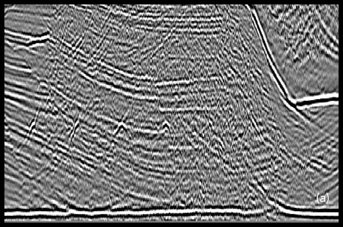
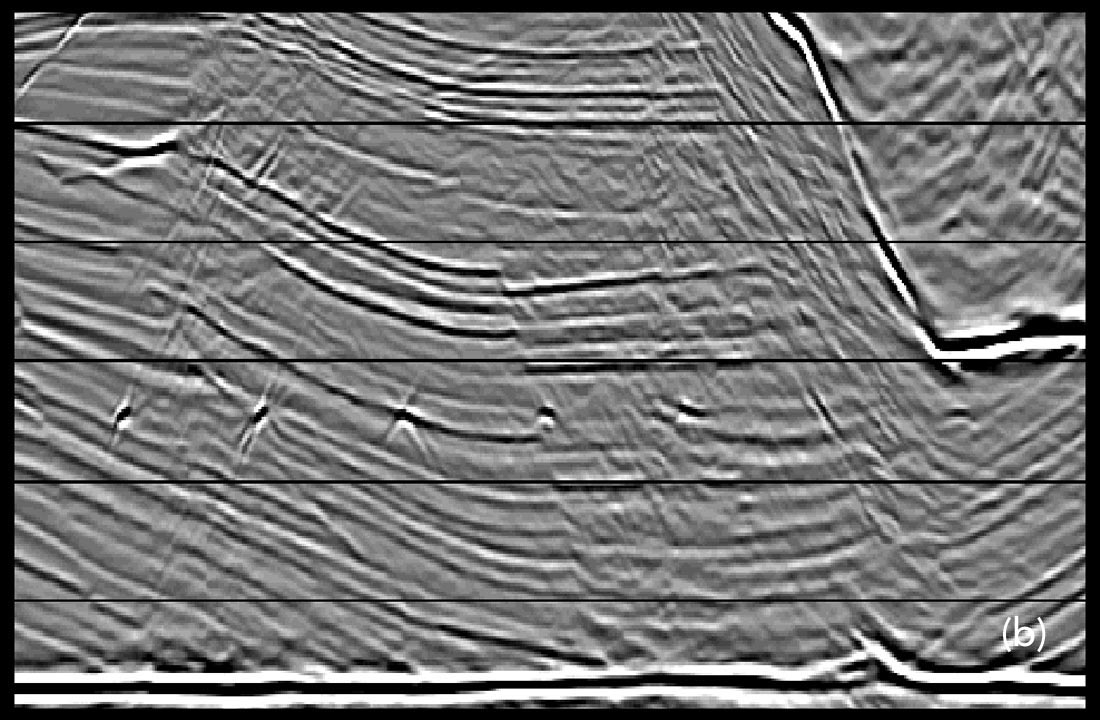
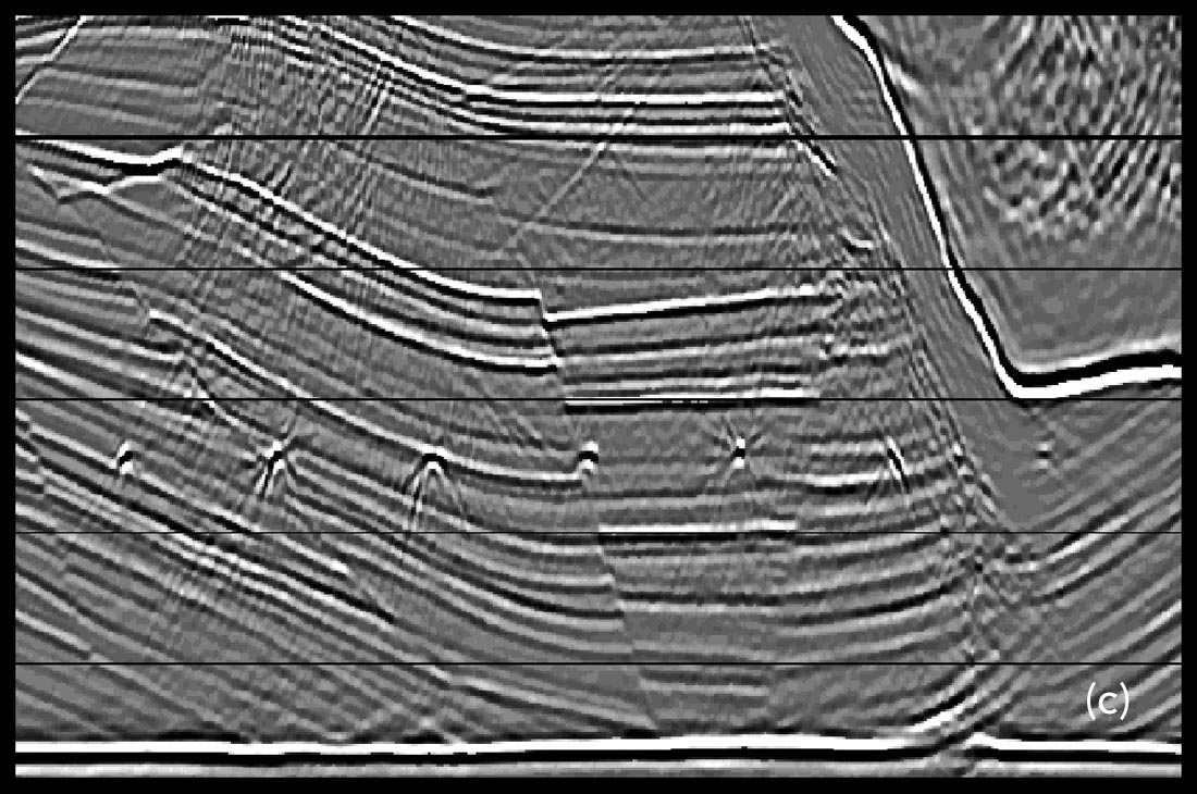
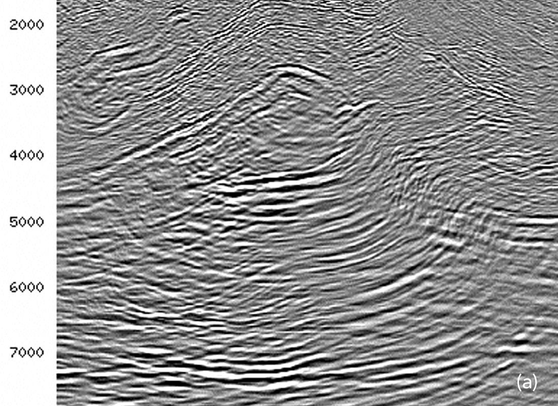
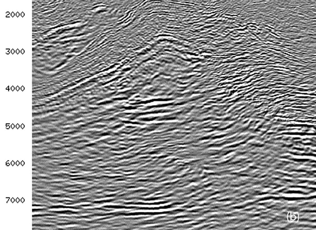
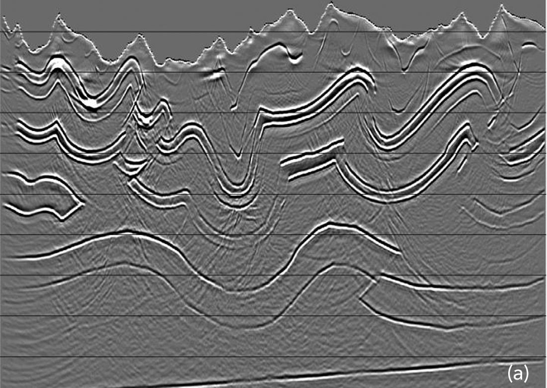
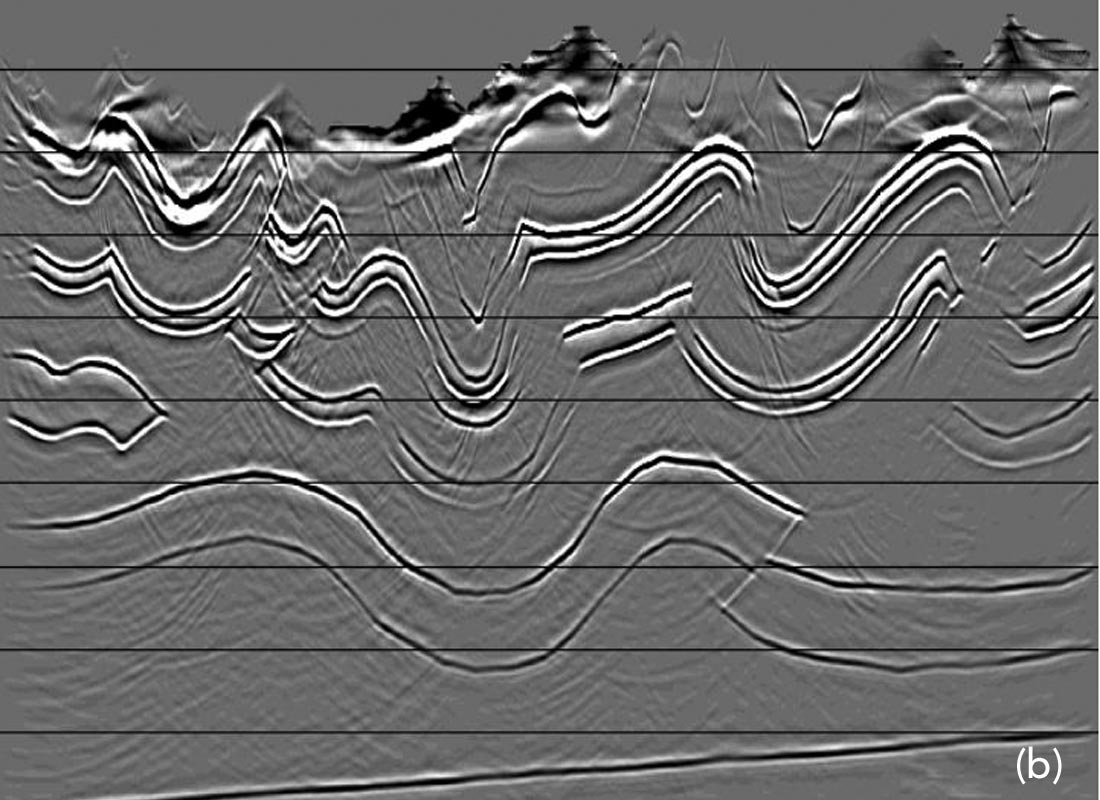
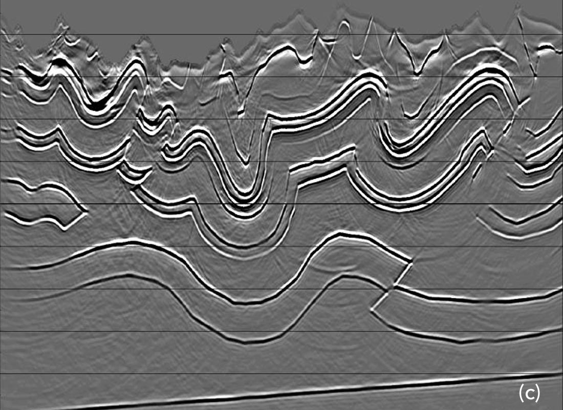
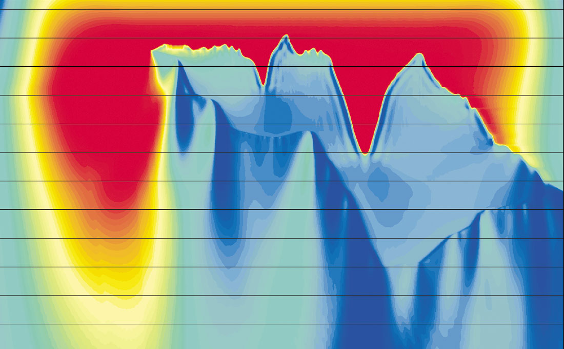
Figures 3 and 4 show comparisons between Kirchhoff migration and the newer methods on two well-known synthetic model data sets. These two comparisons show the range of difference in image quality that we can expect to see in areas of great structural complexity. Figure 3 shows subsalt imaging detail on a marine model (Sigsbee 2a) that features steep canyons incised into a rough top of salt (Figure 6). Steeply-dipping base of salt appears on the upper right side of the images. The Kirchhoff (Figure 3a) image is noisy, and it is hard to distinguish the subsalt fault blocks that are more clearly imaged on the Gaussian beam image (Figure 3b), and very clearly imaged on the WEM image (Figure 3c). Figure 4 shows images from the familiar Amoco model built in 1994 by Gary Maclean. This model features complex structure and very rough topography, typical of many Foothills areas. The Kirchhoff image (Figure 4a) is adequate, showing all the complex structures, but the Gaussian beam and WEM images (Figures 4b and 4c) are significantly cleaner, with less noise and fewer migration smiles.

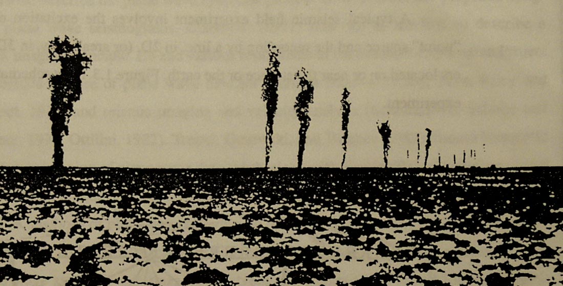
Not only are there new migration methods; there are new, or newly rediscovered, migration domains. WEM methods restrict the types of record they migrate to be wavefields (e.g., common-shot or common-receiver records but not common-offset records). Normally, we see this as a disadvantage relative to Kirchhoff migration, which is comfortable migrating records that are not wavefields (e.g., all traces within a given range of offsets and/or azimuths). But this can work to the advantage of WEM methods, as in the following. A single shot generates a wavefield observed at the receiver locations; a plane-wave source (if it existed) also generates a wavefield observed at the receiver locations, so a “plane-wave” record is a candidate for WEM. Although to my knowledge there has been only one example of such a record generated in a field experiment, shown in Figure 5, these records can be synthesized in processing by an appropriate combination of actual field records. One way of doing this for marine records, used widely at Amoco in years past by Dan Whitmore, is to synthesize delayed shot records, by slant-stacking common-receiver records and posting the results into common-angle sections, with each trace being posted at its receiver location. The result of this is the same as if line sources, with various incidence angles, had been used instead of point sources. These records have a number of advantages over the point-source data that we actually record. There are many fewer of these records than the recorded shot records. They span the entire length of the survey, with no need for padding with zero traces before migration to migrate steeply dipping events far outside the recording aperture. Spanning the entire length of the survey, they keep aperture truncation artifacts from being migrated into the middle of the survey. They provide migrated records that can be sorted into CDP gathers indexed by the incidence angle implied by the delay. Finally, the source cylindrical waves (actually, for a line in a 3-D marine survey, they generate a source wavefield that propagates as a cone in the subsurface) can be used to produce subsurface illumination plots (Figure 6), showing well-illuminated and poorly-illuminated areas. Once we know the subsurface illumination strength, we can put it to use, as illustrated in Figure 7. Specifically, we can compensate the image by dividing (carefully!) the migrated image by the illumination strength. Where the illumination strength is low, this will gain the (also low) migrated amplitudes up to a reasonable level.

In addition to their structural imaging advantages over Kirchhoff migration, both the WEM and beam methods can potentially deliver greater fidelity in dealing both with migration velocities and migrated amplitudes. This can be accomplished by tweaking these methods to produce migrated CDP gathers indexed, not by surface plane-wave angle, but by subsurface opening angle at each image location. These “subsurface angle gathers” will lead to a change in the way we do tomography, and they will lead to more reliable migrated AVA estimates. This development is not yet in common use.

Plane-wave or delayed-shot WEM has become a useful production imaging tool for 3-D marine data, but it will clearly have problems on land. For example, how do we form these records when the near-surface contains significant topographic and velocity variations? How do we perform slant-stacks of poorly sampled 3-D common-receiver records?

Before you step out onto the bleeding edge...

Before you step out onto the bleeding edge, there are a few things you should know.

As I mentioned in the preceding section, delayed-shot WEM has serious problems with 3-D land data. For that matter, so does the more standard common-shot WEM. While Kirchhoff migration can migrate all the traces within a given range of offsets to produce a partial image, common-shot WEM is not so flexible. Migrating a single shot record at a time, WEM will build the complete image by accumulating all the migrated shot records; but none of the individual migrated records will give a satisfying view of geology. Also, the migrated shot records fail to provide the offset information that we find useful for current tomographic velocity analysis and AVO analysis. The final stack will show all the advantages of WEM over Kirchhoff migration, but it will rely on Kirchhoff migration for any tweaks to the velocity field.

A related problem for WEM is that of wavefield sampling. WEM proceeds by “downward continuing” a wavefield into the Earth. Within a live patch for a given shot, the receiver spacing might be a few tens of metres, but the receiver line spacing can easily be on the order of a hundred metres or more, several wavelengths at the highest frequencies. Because of this, these frequencies won’t be able to migrate across receiver lines without aliasing and, as with Kirchhoff shot-record migration, the individual WEM shot-record images will be noisy. As with Kirchhoff shot-record migration, this noise will largely cancel when all the images are stacked into the final image, but the individual shot-record images will not be very useful.

Another problem for WEM shows up when we use it to image very steep dips, especially in 3-D. Except for reverse-time migration, WEM methods that continue a recorded wavefield down into the Earth prefer to look down, not across. As a result, they tend to lose the ability to image the very steepest dips, with the problem being generally worse in 3-D than in 2-D. Worse yet in 3-D, the need to split each downward continuation step into two orthogonal (x,y) steps causes a “splitting error,” which mispositions steep dips in directions oblique to the x- and y-directions.

Finally, anisotropy presents a challenge for WEM. Especially in the Foothills, we have become proficient at estimating anisotropy and incorporating it into our Kirchhoff migration routines (Figure 1). This work took a while, and it had a steep learning curve. Presently, we are at the bottom of a similar learning curve for WEM, with a set of technical (wave-equation) problems quite different from those we solved in our raytracers. Briefly put, anisotropy is a phenomenon of the elastic wave equation, not the acoustic wave equation. Our raytracers manage to fake out the elastic nature of the problem quite nicely under the assumption of weak (or even strong) transverse isotropy, and our one-way acoustic WEM will need to find a different way to fake out the elastic problem. Our present anisotropic capability in WEM is VTI, transverse isotropy with a vertical axis of symmetry.

Will WEM be able to overcome these problems? I am confident that the answer is “yes,” but I must emphasize that the solutions won’t always result from a frontal assault on the problems. For example, sampling theory imposes fundamental uncertainties on imaging wavefields, and straightforward modifications of existing methods won’t make these uncertainties disappear. On the other hand, I predict that the problem of anisotropy will fall more easily.

Are Kirchhoff migration and WEM the only choices? Figures 3 and 4 show Gaussian beam images that compare very well with the WEM images. This method has much of the flexibility and efficiency of Kirchhoff migration and much of the accuracy of WEM. Based on rays, it can image very steep dips without splitting error in 3-D, and can handle anisotropy easily. Also, it can feed very naturally into either today’s standard common-offset tomography or the more advanced velocity analysis methods that the development of WEM will encourage. It is complicated to understand, though, and consequently hard to develop. The beam family of migration methods is currently an area of intensive research, and simplifying principles will emerge, allowing easier understanding and development.

Conclusions

Depth imaging beyond Kirchhoff migration is real, and of real benefit. WEM is widely used in imaging large marine 3-D surveys, and it shows great promise in imaging 2-D Foothills data, but sparse sampling of 3-D Foothills data will limit its full effectiveness for some time. Beam methods, particularly the ray-based Gaussian beam method, will soon be of great use in performing anisotropic depth migration in both 2-D and 3-D.

Acknowledgements

Several of my colleagues contributed most of the work and examples reported here. I especially thank James Sun, Yu Zhang, Rob Vestrum, and Scott Cheadle. Thanks also to Oliver Kuhn for a careful reading.