The anatomy of anisotropic diffusion filters

Summary

This paper provides a detailed analysis of how anisotropic diffusion filters work on seismic data. The conventional trace mixing filter is shown to be an implementation of a specific diffusion process. Diffusion filters have different forms, ranging from the simplest linear isotropic (L-I) diffusion to the most complex nonlinear anisotropic (NL-AI) diffusion. The NL-AI diffusion filter can be considered as the ultimate generalization of trace-mixing. It can be implemented as a structure-oriented filter that follows the expanding direction of each reflection event and enhances its coherency, and stops smoothing when discontinuities are encountered.

Introduction

One of the simplest filters in seismic data processing is trace mixing. The trace-mixing technique is very efficient in enhancing the lateral continuity of horizontal events. It may also reduce the lateral resolution of dipping events and structural discontinuity features. A“smart” filter should be able to recognize the dipping directions of reflection events, and filter the data along those directions. And “smarter” yet, it should also be able to identify discontinuities and stop filtering wherever desired.

The anisotropic diffusion filter introduced to seismic data processing by Fehmers and Hocker (2003) is such a “smart” filter. Fehmers and Hocker (2003) give an excellent description of the implementation of the anisotropic diffusion filter. No redundant discussion will be presented here. The purpose of this paper is to show how diffusion filters evolve from the simplest trace-mixing-like filter to the sophisticated structure- oriented edge-preserving filter.

I first introduce the relation between the linear diffusion equation and the Gaussian filters. Then I show that a discrete implementation of a specific diffusion process ends up exactly the same as the conventional trace-mixing. The later sections show, with some data examples, that diffusion systems with nonlinearity and anisotropy properties are more suitable for filtering seismic trace ensembles.

The discussions here are carried out in the 2-D scenario. The 3-D case is fundamentally similar and will not be discussed here.

Linear diffusion equation, Gaussian filter, and trace-mixing

The diffusion process and seismic recording are both time-related, but the time variables in these two processes have no meaningful relation in the present context. I will use the Greek letter τ for the diffusion process and the Latin letter t in the seismic context.

An ensemble of seismic traces can be considered as an image in the x-t domain or as a two-variable function u(x, t). Assume such an image or function represents a status snapshot of some starting or on-going diffusion process. When the diffusion process goes on, the function values change and different images, u(x, t, τ), evolve at later times τ. These later snapshot images can then be put back into the seismic context and become different versions of the filtered seismic traces.

A linear diffusion process can be expressed by the following equation,

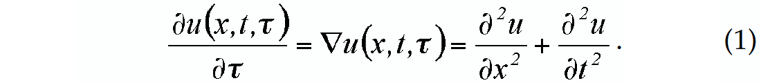
If a initial status u(x, t), such as the input seismic section, is known, the solution of equation (1) at later diffusion time τ is proved to be the same as the convolution of u(x, t) with the 2-D Gaussian kernel of the form

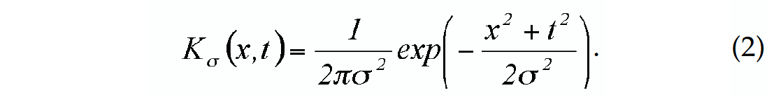
where σ² = 2τ (Weeratunga and Kamath, 2003).

The diffusion process described by (1) is therefore equivalent to some time and space domain filter with Gaussian window functions. Intuitively, larger σ makes the Gaussian filter stronger, and longer-time diffusion will also balance out more of the differences of the properties being diffused. Such Gaussian filters are not the most popular filters used in seismic data processing because they need spatially unlimited operators. However, discrete implementations of the diffusion filters can be spatially and temporarily limited, and they can be very convenient for practical applications.

Let’s examine a simple case of the problem. Assume there is no diffusion in the t-direction, so the diffusion at any time t₀ becomes a 1-D process

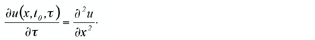
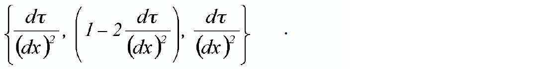
If the status function at τ is known, the solution at (τ+dτ) can be expressed numerically with a straightforward finite-difference scheme as

or

This is a three-point mixing filter with operator

Equation (1) is a linear isotropic (L-I) diffusion equation. The word “ isotropic” is used to emphasize the differences from a series of more complicated diffusion processes discussed in the next section. Their correspondingly more complicated mathematical equations will not be explicitly discussed in this paper. More general forms of anisotropic diffusion equations can be found in Fehmers and Hocker (2003) and Weeratunga and Kamath (2003).

Evolution of diffusion equations

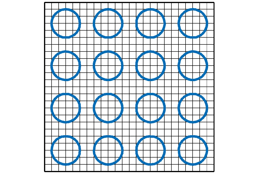
The diffusion process described by equation (1) has the properties of (i) linearity, the diffusion filter strength at all the locations is the same, and (ii) isotropy, the diffusion filter strength in different directions at any location is the same.

The standard deviation of a Gaussian determines its shape and represents the strength of its related Gaussian filter. In general, the larger the standard deviation, the stronger the Gaussian filter. Figure 1 uses the radii (of the circles) to represent the value of the standard deviation of the Gaussians. The circles themselves represent the “isotropic” property of the diffusion process, i.e., the Gaussian filter at each location has the same strength in all directions. The linearity is reflected by the uniform size of all the circles.

As a one-dimensional filter, trace-mixing does not relate to the concept of diffusion direction (there is only one direction involved). Trace- mixing filters are usually implemented as “linear” diffusion filters with their operator (triangle or boxcar) fixed for all locations. Trace-mixing filters can also be implemented as “nonlinear”, with neighbouring traces mixed with different weights at different locations.

A general nonlinear isotropic (NL-I) diffusion process can be illustrated as in Figure 2. Compared with Figure 1, a nonlinear filter can have different filter strengths at different locations, and this is shown by the different-radius circles in Figure 2. The Gaussian filter kernels are still represented by circles since the “isotropy” property is maintained.

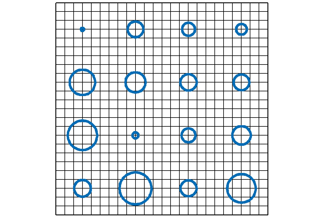
The idea of nonlinear filtering is the starting point of edge-preserving smoothing techniques. A quantified edge-likelihood can be used to control the filter strength and prevent image edges from smoothing over. The edge-preserving diffusion filtering of seismic data is extensively discussed in Fehmers and Hocker (2003), and it will be further discussed in this paper later.

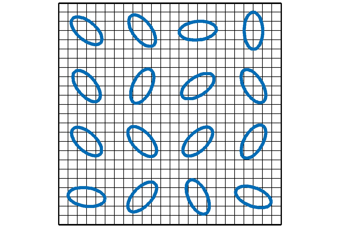
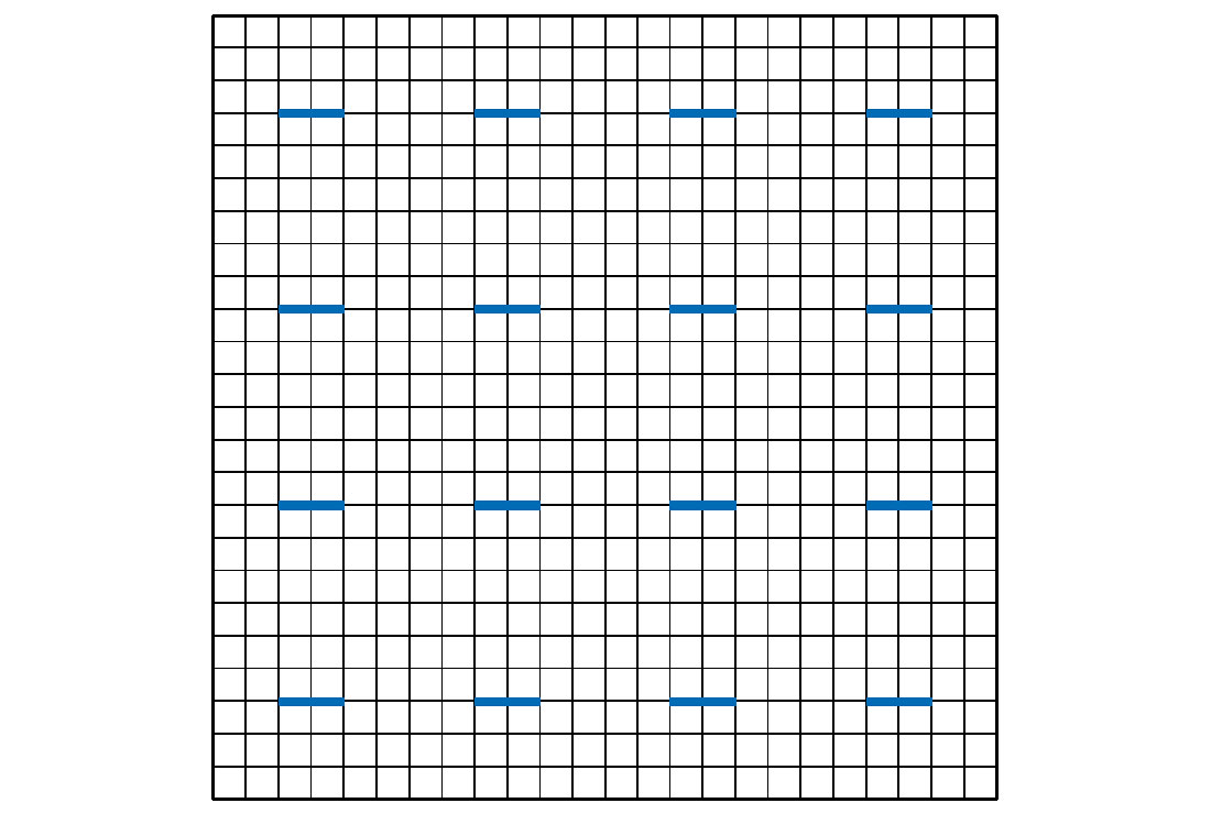
Another intermediate evolving stage is the linear anisotropic (LAI) diffusion equation. Such diffusion processes allow different strengths in different directions at each location but remain the same total filter strength for all the locations. Figure 3 shows the general scheme of L-AI diffusion processes, where the anisotropy property is shown by the oval-shaped kernels (other than circles). The linearity is reflected by the uniform size of the ovals at all locations. This combination of relaxation and restriction (allowing anisotropy but limited to linearity) seems awkward and unpractical. However, the conventional trace mixing, considered as a 2-D filter, is just a discrete implementation of an extreme case of the L-AI diffusion filters. Figure 4 shows the diffusion scheme that governs the trace mixing filter. The ovals in Figure 3 are now reduced to infinitesimally thin, horizontal, same length line segments. The anisotropy is reflected by mixing only in the spatial direction, and the linearity is reflected by the same segment length. The Van Gogh filter (Fehmers and Hocker, 2003) is also an example of L-AI diffusion filter. At each location, a Van Gogh filter prefers a certain direction to others in terms of filtering strength, which is the appealing part of this filter. Fehmers and Hocker (2003) combine an edge-detection algorithm to overcome the linearity limitation of the Van Gogh filters and make them more suitable for the filtering of structured seismic sections.

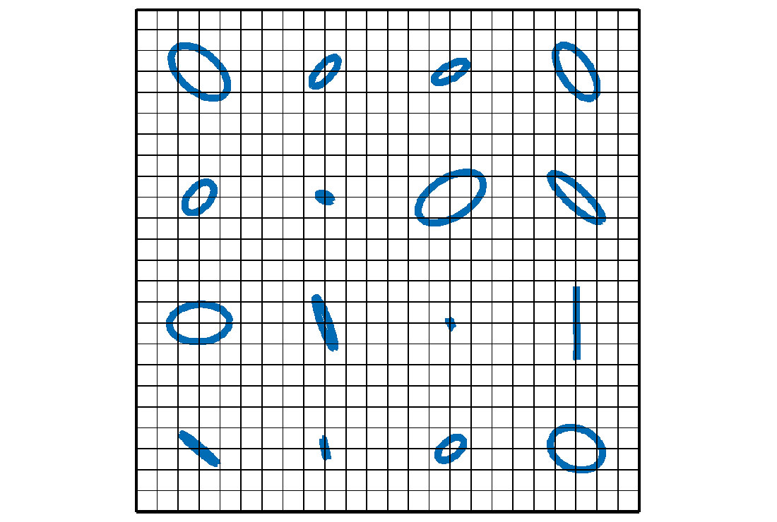
Nonlinear anisotropic (NL-AI) diffusion filters are more suitable to applications on seismic data. Seismic trace ensembles are naturally anisotropic in terms of the different treatments of the sampling issues in time and spatial directions. Most of the multitrace filtering methods are designed to keep the vertical resolution of the traces while enhancing the spatial coherency of the reflection events. Besides, almost all the seismic recordings contain events with different dips. It is important for an efficient filter to be able to recognize the dips and enhance the continuity of the dipping events accordingly. On the other hand, it is also desirable to have a filter whose strengths can be adjusted based on the local surroundings of the trace samples. Not only should the filter properly enhance the continuity of coherent events but it should also be able to reduce the filter strength to prevent from smearing meaningful discontinuity features. Figure 5 illustrates the scheme of a general NL-AI diffusion process where the sizes and shapes of the Gaussian kernels vary with locations.

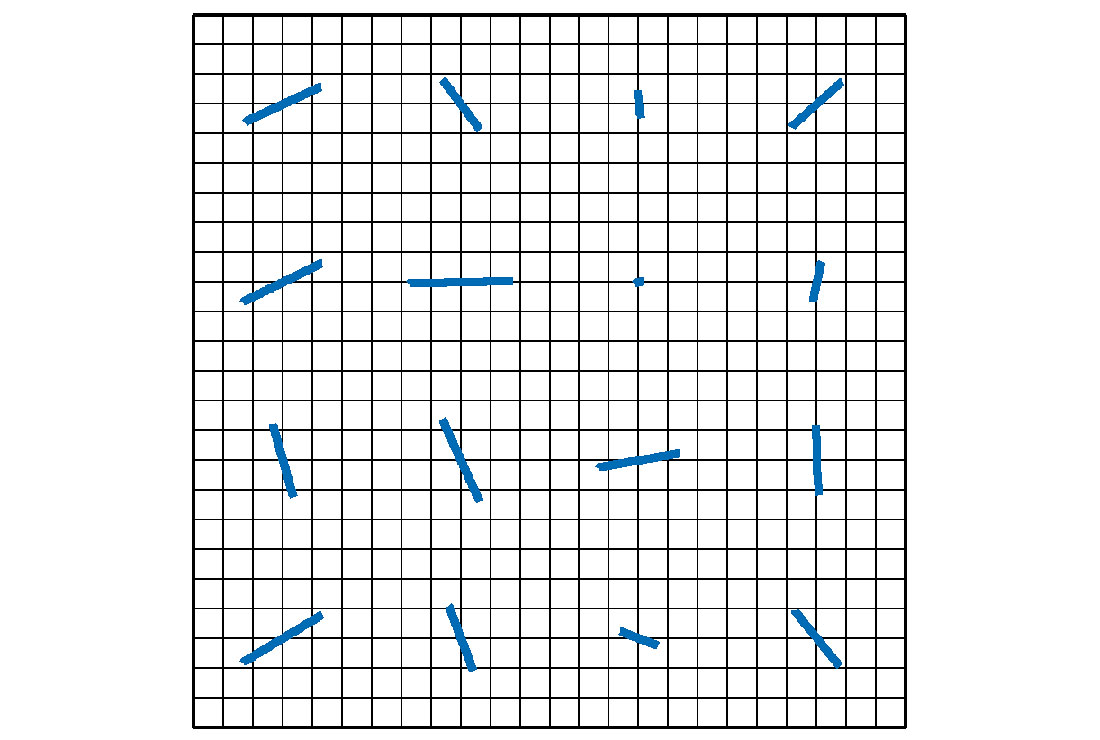
Designed as a structure-oriented filter, the NL-AI diffusion filter is expected to “smooth” the reflection events along the events’ expanding directions. Any smoothing in other directions will no doubt reduce the resolution of such events and therefore is not encouraged. When the expanding direction of an event is found, the diffusion can only proceed in that direction. Such a special case of nonlinear anisotropic diffusion filter is illustrated in Figure 6. Compared with Figure 5, the oval shaped kernels are now reduced to line segments. The lengths of the segments represent the filter strengths, and the line directions are the only directions along which the diffusion happens. Comparing Figure 6 with Figure 4, which depicts the conventional trace mixing filter, one can consider the final version of the NL-AI diffusion filter is a generalization of the trace-mixing technique.

Discontinuity detection for seismic sections

Noise attenuation or continuity enhancement filters often reduce some resolution power of seismic data by smearing the discontinuities. The edge detection technique can be borrowed from digital image processing literature to identify and quantify the discontinuities on a section. The quantified discontinuity can then be used to control the filter strength in the diffusion process.

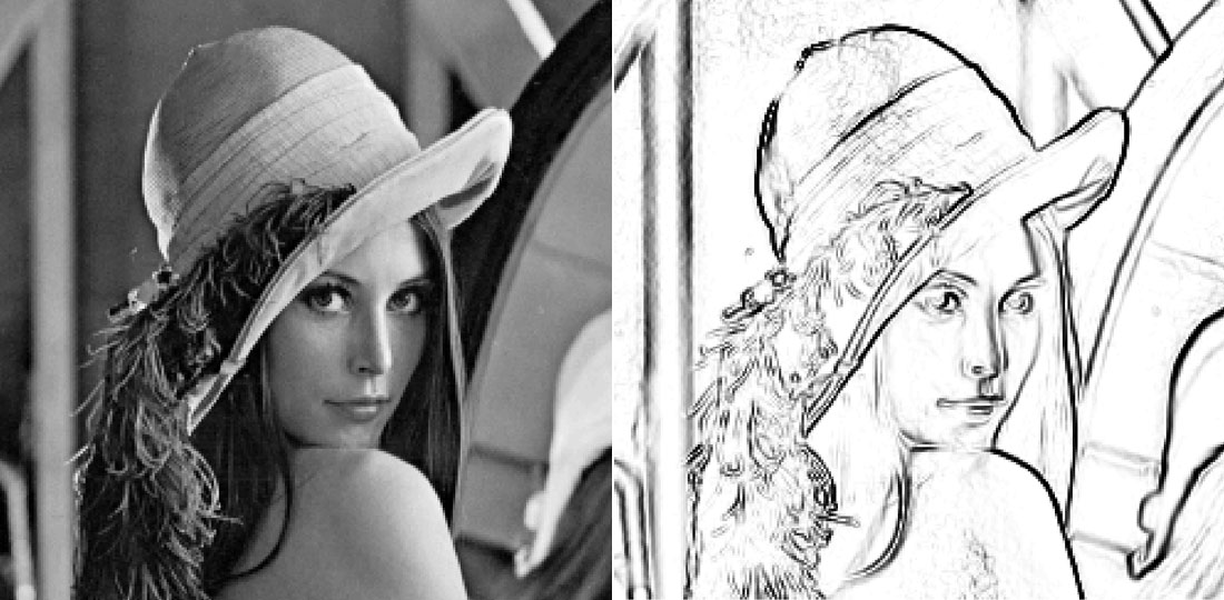
In image processing, “edge” as a quantity can be defined as the sudden changes in a digital image. Such edges often need to be treated differently than other places in an image. Edge detection has been a hot topic for image processing. One type of widely used edge-detection algorithm is based on gradient magnitudes along different directions. These algorithms are fairly efficient in detecting the edges of digital images. Figure 7 shows a picture (a) and its edges detected by a gradient based algorithm (b). Note that the detection result almost perfectly identified all the visible edges. Experiments of these edge detection methods on seismic data, however, show that the most common edges detected are the zero-crossings. Zero-crossings are seldom considered “edge” in seismic data. They are mostly part of the continuous events.

The edges important to seismic processing and interpretation are discontinuities of reflection events that are geophysically meaningful. What we need is a discontinuity detection algorithm. The edge detection algorithm from Fehmers and Hocker (2003) is based on differences resulted from the applications of different-size smoothing operations, and it works efficiently to identify the discontinuities in seismic data. The quantified discontinuities can be used to determine the diffusion strengths. In the extreme cases, when a discontinuity is detected with high confidence, no filtering should be applied; and when no discontinuity is detected, the full strength filter should be applied. Different interpolation functions can be used to smoothly connect the two extreme cases.

Examples and discussions

For data without apparent structure or dipping events, NL-AI diffusion filters perform well as a coherency enhancement and random noise attenuation filter. The filtered results are comparable to those filtered by f-x decon or trace-mixing. Numerous applications to seismic data from the plains area prove the efficiency of nonlinear anisotropic diffusion filters in this scenario.

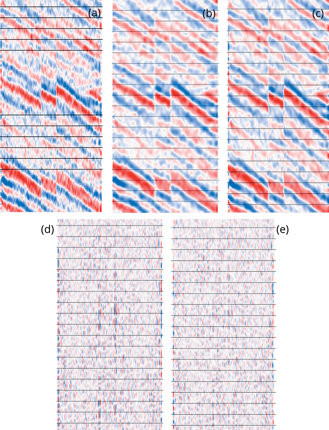
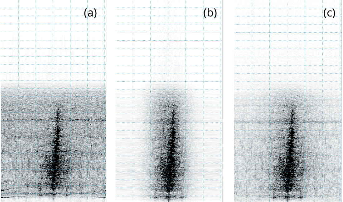
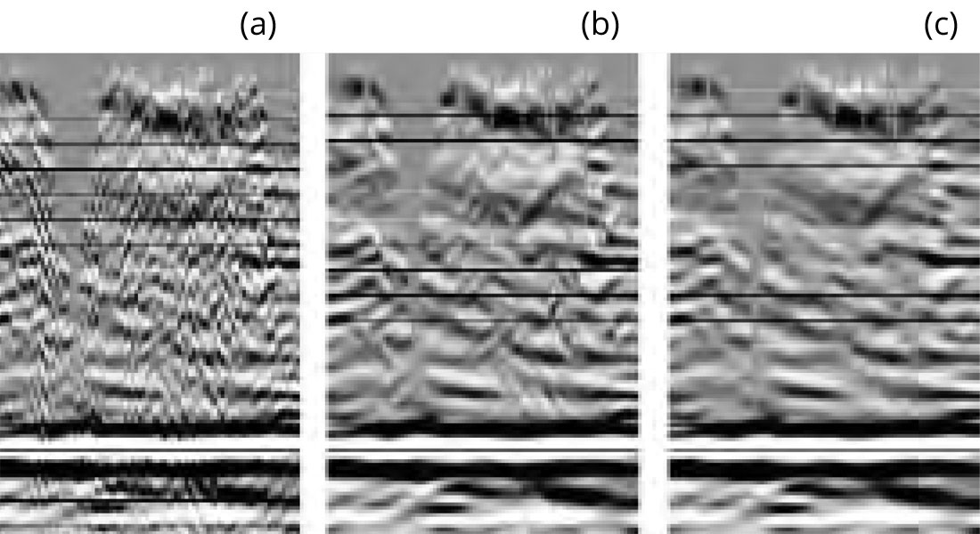
The NL-AI diffusion filters show their advantages over conventional trace-mixing filters when the seismic sections contain dipping events and/or discontinuities. Let’s examine the results of filtering a synthetic section where some real seismic traces are static shifted to create systematic dipping events and vertical fault-like discontinuities. Figure 8 (a) shows a portion of the stack. Figure 8 (b) is the same stack but filtered by trace mixing and (c) is the stack filtered by a NL-AI diffusion filter. Both (b) and (c) have much less noise and their events are more coherent, as expected. In order to see the difference between (b) and (c) and realize the superiority of the NL-AI diffusion filter, two difference sections are created. One is the difference section from (a) to (b), shown in Figure 8 (d), and the other is the difference from (a) to (c), shown in Figure 8 (e). Both difference sections (d) and (e) contain mostly incoherent noises, even though the difference section (d) does contain more energy than (e). The most noticeable coherent energy shown in (d) corresponds to the vertical faulting edges, where in (e) the difference is much weaker. This means the trace mixing may have smoothed more than necessary near the discontinuities. If this discontinuity is meaningful, the trace-mixing result will be less plausible. Figure 9 shows the fk spectra of the three sections shown in Figure 8 (a), (b), and (c), respectively. The energy at large wavenumbers on Figure 9 (b) is much weaker than that shown in Figure 9 (c). This implies that the trace mixing may have lost more lateral resolution than necessary, and this is undesirable.

The shallow parts of seismic sections often contain many kinds of noises. Besides the random noise, coherent noises such as residual ground- roll, refraction energy and even acquisition footprint, are often present at the top of the seismic sections. The computation of event expanding rections can be noise sensitive, caution is needed when more than one direction present at same locations. The following example shows one way to overcome such contradictions. To reduce the sensitivity to the noise, the dip detection operators are smoothed over a certain spatial range. The size of this smoothing range should be left adjustable to accommodate the noise level of the data. Figure 10 shows the shallow portion of a stacked section (a) and the filtered results, (b) and (c) used two different selections of the smoothing operator size. The larger smoothing size operator (15 samples in each direction) used for (c) tends to stabilize the local dip detection, and the major background dipping trends stand out of the local noisy dips.

Readers who would like to see more results from the diffusion filter are referred to Fehmers and Hocker (2003). It can be used as an alternative to other coherency enhancement and random noise attenuation methods. It is very efficient for cleaning up stack sections, migrated or not. While for migrated stacks, it is recommended to use the edge-preservation version of the diffusion filter. If there are events with conflicting dip directions, this filter should be used cautiously.