A Summary of Several Challenges Facing Multi-Parameter Elastic Full Waveform Inversion

In spite of all that there is still to learn about seismic full waveform inversion (FWI), and there is a lot, the technology has accumulated some significant success stories in recent years – enough to motivate researchers to think quite ambitiously about how far we might go with it. Moreover, FWI has at its core an admirable organizing principle, one which should be a key driver of all seismic technology development, namely: “our data are measurements of a wave field, and we should treat them that way.” Without in any way suggesting that it will be easy to do so, our group has put quite a bit of effort into understanding how this philosophy can be realized practically at the reservoir scale, producing practical and robust determinations of multiple elastic parameters. The purpose of this article is to briefly grapple with some critical aspects of multi-parameter FWI. In particular, we ask: What are the key ingredients of a FWI flow? How do we calculate them given reasonable computational resources? How are several elastic parameters simultaneously determined from seismic measurements?

FWI makes maximal use of wavefield information to invert subsurface elastic parameters by iteratively minimizing the differences between the modelled data and the observed data. Compared to traditional seismic inversion strategies, FWI methods have many advantages but also experience a set of difficulties for industrial applications, including slow convergence rate, lack of low frequencies, and extensive computational burden.

Traditional optimization methods for FWI in exploration geophysics are gradient-based (i.e., steepest-descent (SD) and non-linear conjugate-gradient (NCG) methods). By ignoring the contributions from the second-order derivative of the misfit function (namely the Hessian operator), these gradient-based methods are computationally attractive for large-scale inverse problems, however, they suffer from slow convergence rates (Pratt et al., 1998; Pan et al., 2014; Pan et al., 2015a). The Hessian operator can greatly enhance the search direction by compensating for geometrical spreading, mitigating finite frequency effects, and suppressing the parameter cross-talk problem. However, explicit calculation, storage, and inversion of the Hessian are computationally impractical for large-scale inverse problems. Quasi-Newton methods (e.g. the L-BFGS method) approximate the inverse Hessian iteratively by storing the model and gradient changes from previous iterations (Nocedal and Wright, 2006).

Hessian-free optimization methods (truncated-Newton methods) represent attractive alternatives to the above-described optimization methods (Santosa and Symes, 1988; Metivier et al., 2012; Pan et al., 2016b; Pan et al., 2016c; Pan et al., 2016d). Instead of constructing the Hessian explicitly, only Hessian-vector products are required. At each iteration, the search direction is computed by approximately solving the Newton equations using a conjugate gradient algorithm. In this paper, we show the quadratic convergence provided by the second-order optimization method and discuss its benefits in suppressing parameter cross-talk in multi-parameter FWI.

The ideas and quantities of multi-parameter seismic FWI

Full waveform inversion proceeds by defining a misfit function, which takes any Earth model as input, and returns a single positive number as output. The function Φ must be so designed that when the input Earth model is as close as it can come to the actual Earth model below our feet, the number returned is a minimum. This transforms our problem to the problem of finding the minimum of Φ. Typically, the misfit for FWI is defined as:

where ‖.‖² indicates the square of L-2 norm, m is the model parameter vector, d_obs and d_syn are the observed data and synthetic data respectively. This is a data validation scheme: we are satisfied with our candidate Earth model when the data we predict from it is as close as possible to the data we measured in the field. To minimize the quadratic approximation of the misfit function, the model can be updated iteratively:

where Δm_k means the search direction at the kth iteration and μ_k is the step length, which can be obtained with a line search method. Within Newton optimization framework, the search direction is the solution of a Newton linear system:

where g_k is the gradient vector, the first derivative of the misfit function and H_k is the Hessian operator, the second derivative of the misfit function, which carries crucial information in the inversion process:

where the symbols † and * indicate transpose and complex conjugate respectively, and ∆d is the data residual vector. The first term of equation is known as Gauss-Newton Hessian approximation which represents first-order scattering effects. In multi-parameter FWI, the parameter cross-talk arising from the coupling effects between different physical parameters make the inverse problem more undetermined. The multi-parameter Gauss-Newton Hessian has a block structure. The off diagonal blocks are expected to decouple different physical parameters (Operto et al., 2013; Innanen, 2014; Pan et al., 2016a).

The simplicity of equations 1-4 belies the computational effort required for each iteration. There are a range of “flavours” of FWI update, differentiated by how computationally intensive they are; the cost of a computationally cheaper iteration being that convergence rates decrease and phenomena such as cross-talk increase. In the SD method, the search direction is the negative of the gradient vector. In non-linear conjugate gradient method, the search direction is just the linear combination of the gradient with previous search direction. The L-BFGS method approximates the inverse Hessian by storing the model and gradient changes from a number of M previous iterations. Hessian-free Gauss-Newton (HFGN) method only requires Gauss-Newton Hessian-vector product v (v is an arbitrary vector), which can be calculated using the adjoint-state technique. At each iteration, the search direction is obtained by solving the Newton equation iteratively with a conjugate gradient algorithm. A L-BFGS preconditioning strategy can be employed to accelerate the HFGN method (Pan et al., 2016c).

Some simple examples

In this section, we begin by exemplifying some of the trade-offs and possibilities the optimization methods discussed above afford. In particular, we focus on the quadratic convergence rate of the HFGN method in single parameter FWI. Then, we consider the special issues arising from multi-parameter FWI. Specifically, numerical examples are given to illustrate the efficiency of the multi-parameter Gauss-Newton Hessian in, and the consequences for, simultaneous determination of the elastic parameters.

Comparison of different optimization methods

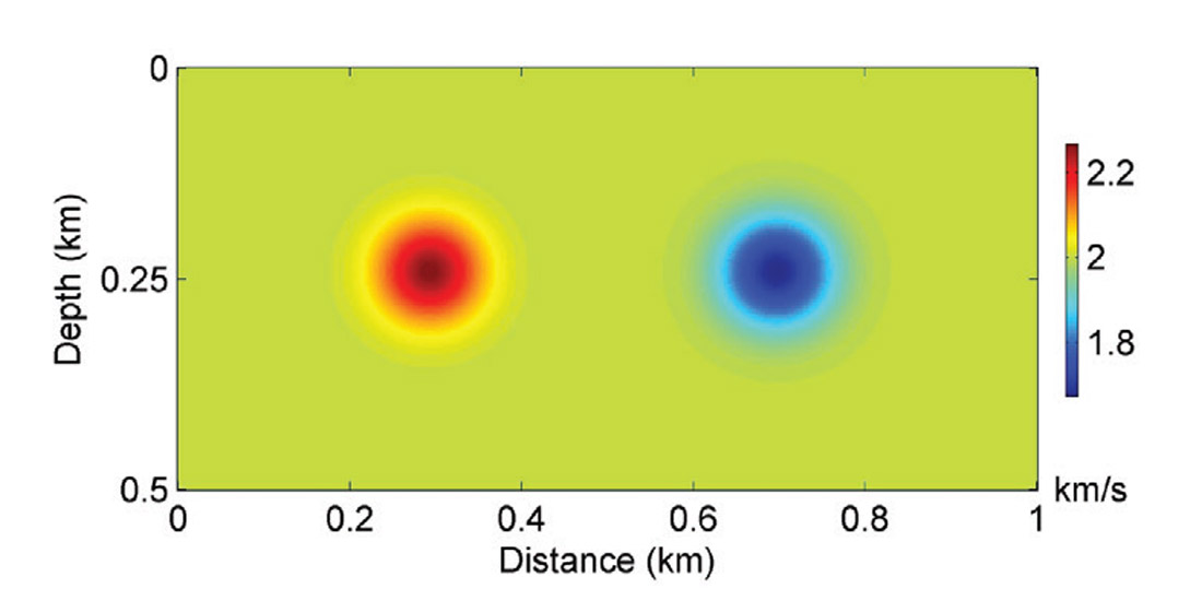
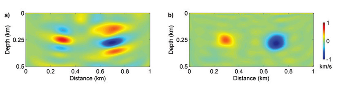
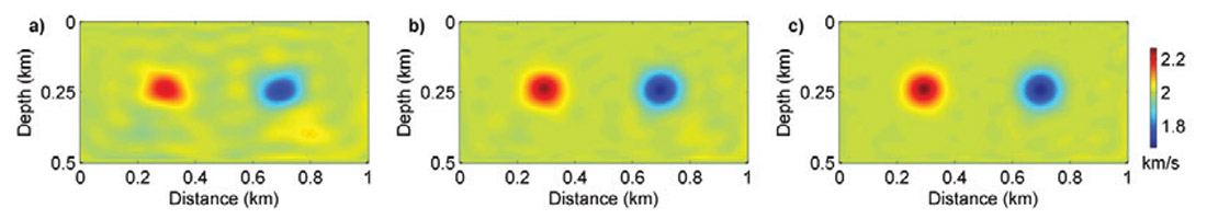
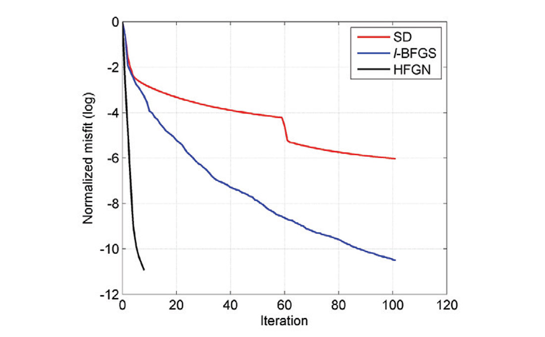
Figure 1 shows the true velocity model with two Gaussian anomalies. The initial model is homogeneous with a constant velocity of 2 km/s. Forty-nine sources and one hundred receivers are distributed regularly at the top surface of the model. Figures 2a and 2b show model updates for the SD and HFGN methods with 30 CG iterations. As we can see, with the Gauss-Newton Hessian, the model update is clearly de-blurred. Figures 3a, 3b and 3c illustrate the inversion results using SD, L-BFGS, and HFGN methods. Figure 4 shows the convergence histories of these three different methods. L-BFGS method converges faster than the SD method and provides a higher quality inversion result. The HFGN method provides a quadratic convergence rate, which is much faster than the SD and L-BFGS methods.

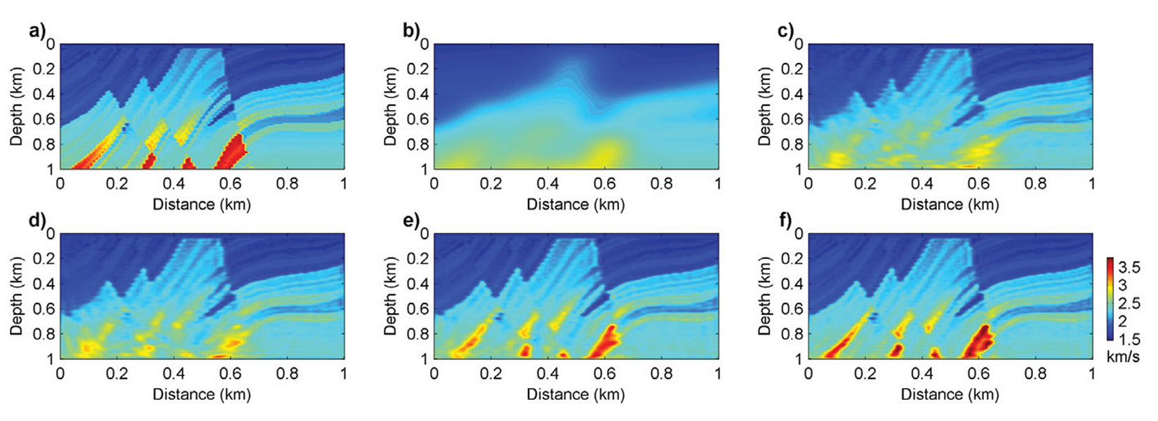
We next examine the advantages of the second-order optimization methods using a more complex model. Figures 5a and 5b show the true velocity model and the initial velocity model. Forty-nine sources and fifty receivers are deployed on the surface with a depth of 20m. The frequencies used for the inversion are increased from 5 Hz to 30 Hz, and include a partial overlap-frequency selection strategy, where a group of 3 frequencies are used for inversion simultaneously. Figures 5c, 5d and 5e are the inverted models using the SD, L-BFGS and HFGN methods. The SD and L-BFGS methods cannot recover the deep parts of the velocity model well. The deep parts of the inversion result obtained using the HFGN method have been obviously enhanced. The HFGN method can be accelerated by appropriate preconditioning strategies. Figure 5f shows the inverted model using a L-BFGS preconditioned HFGN method. As we can see, the inversion result using preconditioned HFGN method is further improved.

Suppressing parameter cross-talk using multi-parameter Gauss-Newton Hessian

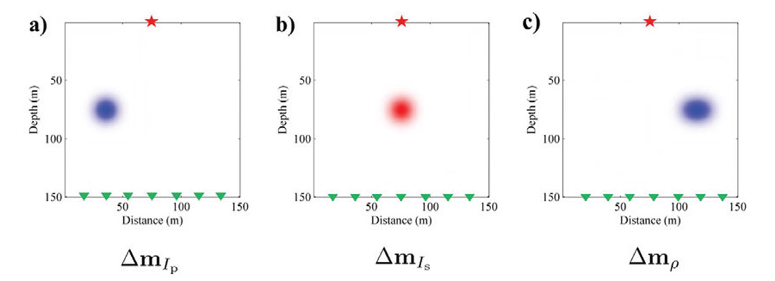
In this section, we present numerical examples to show that the multi-parameter Gauss-Newton Hessian can suppress parameter cross-talk in multi-parameter FWI. We describe the isotropic and elastic media using three parameters: using three parameters: P-wave impedance I_P, S-wave impendance I_S and density ρ. Figures 6a, 6b and 6c show the true model perturbations of I_P, I_S and ρ with three Gaussian anomalies. One source is arranged at the top surface and thirty receivers are distributed at the bottom of the model.

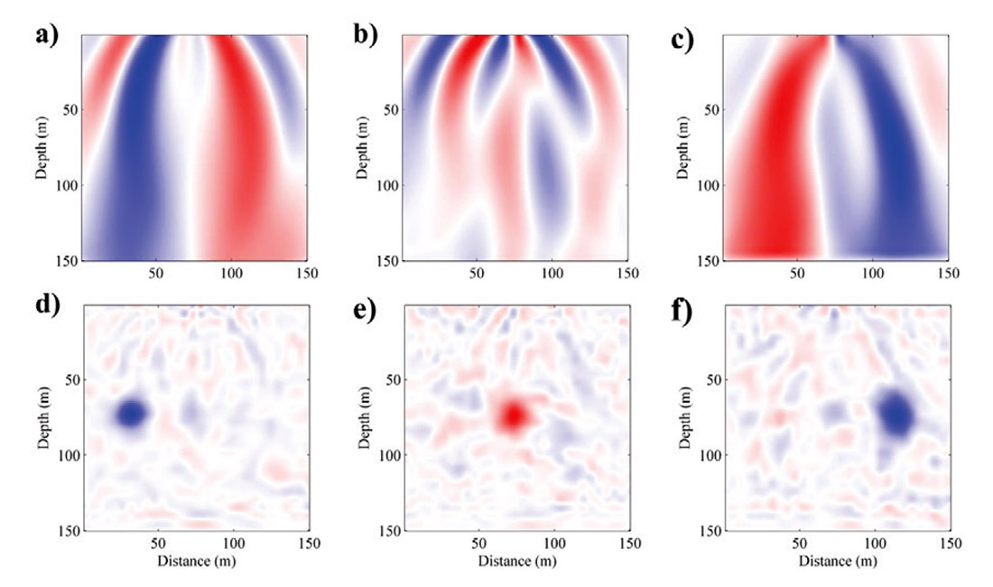
In this numerical example, we examine the advantages of the second-order optimization method by constructing the multi-parameter Gauss-Newton Hessian explicitly. Figures 7a, 7b and 7c show the gradient updates for P-wave impedance, S-wave impedance and density. The model updates are obscure. The density perturbation causes artifacts in the gradient of P-wave impedance and vice versa. Figures 7d, 7e and 7f show the corresponding model updates preconditioned by the multi-parameter Gauss-Newton Hessian. With preconditioning, the model updates are obviously resolved and the artifacts caused by parameter cross-talk are suppressed effectively.

Conclusions

In this paper, we introduce the Hessian-free Gauss-Newton optimization method for full-waveform inversion. The quadratic convergence rate of this second-order optimization approach is illustrated with numerical examples. The role of Gauss-Newton Hessian in suppressing parameter cross-talk is revealed. For further study, a preconditioned Hessian-free Gauss-Newton method for multi-parameter FWI will be developed.

Acknowledgements

This research was supported by the Consortium for Research in Elastic Wave Exploration Seismology (CREWES) and National Science and Engineering Research Council of Canada (NSERC, CRDPJ 461179-13). Wenyong Pan is also supported by a SEG/Chevron scholarship and an Eyes High International Doctoral Scholarship.