Introduction
Synthetic seismograms are critical in understanding seismic data. We rely upon them for an array of tasks, from identifying events on seismic data to estimating the full waveform for inversion. That said, we often create and use synthetic seismograms without much thought given to the input log data or erroneous synthetic results. Contrary to popular belief, and despite how we treat them as interpreters, log measurements are not ground truth, and not all synthetic seismogram algorithms are created equal. Have you ever created a synthetic seismogram that has a tenuous tie to seismic? Have you wondered why the synthetic seismogram changes significantly when the density curve is included? Have you queried the quality of the sonic and density logs used to generate your synthetic seismogram? Have you seen a synthetic seismogram change when a different software package is used? If you can answer yes to any of these questions and / or you would agree that synthetic seismograms are not always simple in your world, then this is the article for you.
We present the nuts and bolts of synthetic seismograms from the perspective of the seismic interpreter; we look at what can go wrong, what does go wrong, and what you can do to prevent falling into some of the pitfalls that arise.
According to the Schlumberger Oilfield Glossary, a synthetic seismogram is defined as:
“The result of one of many forms of forward modeling to predict the seismic response of the Earth. A more narrow definition used by seismic interpreters is that a synthetic seismogram, commonly called a synthetic, is a direct one-dimensional model of acoustic energy traveling through the layers of the Earth. The synthetic seismogram is generated by convolving the reflectivity derived from digitized acoustic and density logs with the wavelet derived from seismic data. By comparing marker beds or other correlation points picked on well logs with major reflections on the seismic section, interpretation of the data can be improved.
The quality of the match between a synthetic seismogram depends on well log quality, seismic data processing quality, and the ability to extract a representative wavelet from seismic data, among other factors. …”
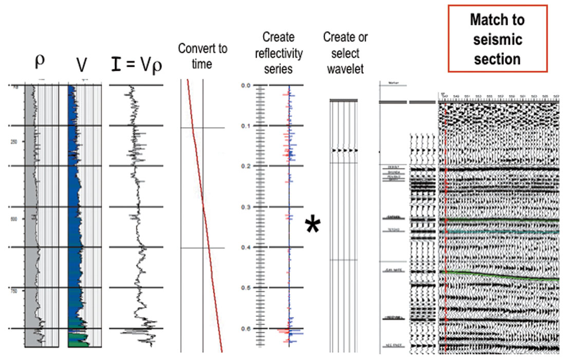
The basic process of creating a synthetic is simple (Figure 1) and described in many geophysical text books, however it is in the details that problems occur. Input density and sonic logs are multiplied together to obtain an impedance log. This a wavelet to obtain the synthetic seismogram. In the Schlumberger definition presented above, we have highlighted some of the inputs and steps that can have problems and/or complications. Keep in mind that doing everything “correctly” can still lead to issues at any or all of the above steps. Below, we discuss a few pitfalls we have witnessed.
Density and Sonic Logs
As geophysicists, we often assume that the well information, particularly log data, provided by our geologist or petrophysicist is the “ground truth”. Nonetheless, we often find high amplitude events in our synthetic seismograms that do not correlate to geology. A common “fix” is to throw out the density log, and build synthetics without it. Depending on the software we use, that means the density is approximated with a constant, or with some pre-defined regression to the sonic log. In either case what we have done is declare the entire density log to be unfit, without really understanding the full picture. An old proverb declares that the devil is in the details. In this case, it turns out, like so often in geophysics, the details are a QC issue.
Density logs are greatly affected by borehole conditions such as washouts or invasion. Reliable density log measurements of the rock require good pad contact with the borehole wall. Without good pad contact, density log measurements will be spuriously low. A geologist or petrophysicist may indicate that the density log is “fine” over the zone of interest. “Fine” is a subjective term. The subjectivity is related to the purpose of the log. If one is simply looking for porosity, then the presence of a washout may indicate porosity, and the log is then suitably “fit for purpose”. If one needs a reasonably accurate measurement of the rock’s bulk density, in order to build a representative synthetic seismogram, then a washout zone is definitely not “fit for purpose”. Geophysicists must be clear with their professional colleagues: “fit for purpose” requirements vary.
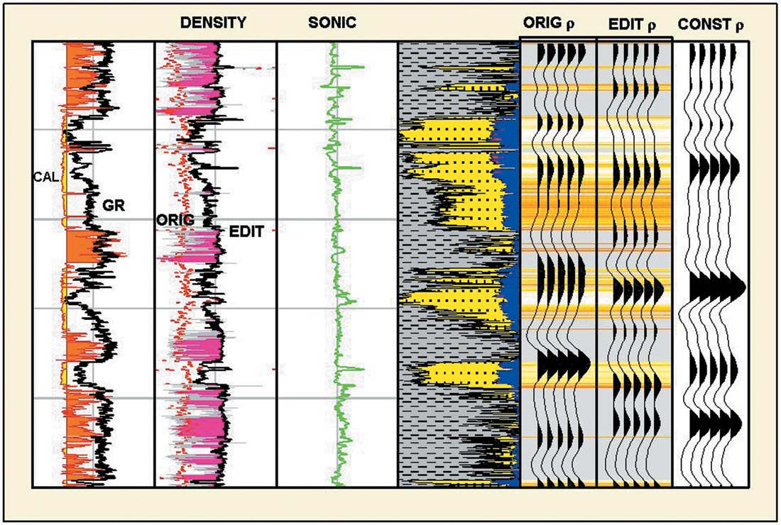
Simply discarding the density log may not be the best procedure, as it may lead to erroneous correlations or phase assumptions. Discarding the entire log implies that we have concluded that the entire log is free of any meaningful content. This is clearly not the case. A better option may be to regenerate the density log over affected intervals using all available supplemental information, although we suggest that this is best left to a petrophysicist. Figure 2 shows an example of a synthetic created using velocity * “raw density”, velocity * “edited density”, and velocity only (constant density), where velocity is calculated from the sonic log. Differences exist between all three, leading to potentially different interpretations of which events correspond to the tops of the sands.
Despite being less sensitive to borehole conditions, sonic logs can also have issues. Sonic logs are measured over a much larger interval, with redundancies built in to most units. Additionally, sonic logs are the result of a process similar to first-break picking on conventional seismic data, essentially the result of picking the time of the direct arrival on several receivers, and computing the time it takes energy to travel from the source to each of the receivers, spaced over several meters. In the end, sonic logs appear to be better behaved because they effectively average over a much larger interval than density. The easiest thing we can do to check the logs is to look at a caliper log. This will give you an indication of the potential for poor readings and where the synthetic amplitudes are suspect. Additionally, this information can be used with additional logs and/or wells to reconstruct the poor log values over that interval, providing a means of creating a more reliable synthetic trace. However, such replacement techniques must be used with care. If a section of log is “bad” in a well this suggests something about the rock properties in this part of the well. If this is replaced by “good” section of log from a different hole, then it may be that the log was only good because the rock properties were different in the other well, and therefore not an appropriate replacement.
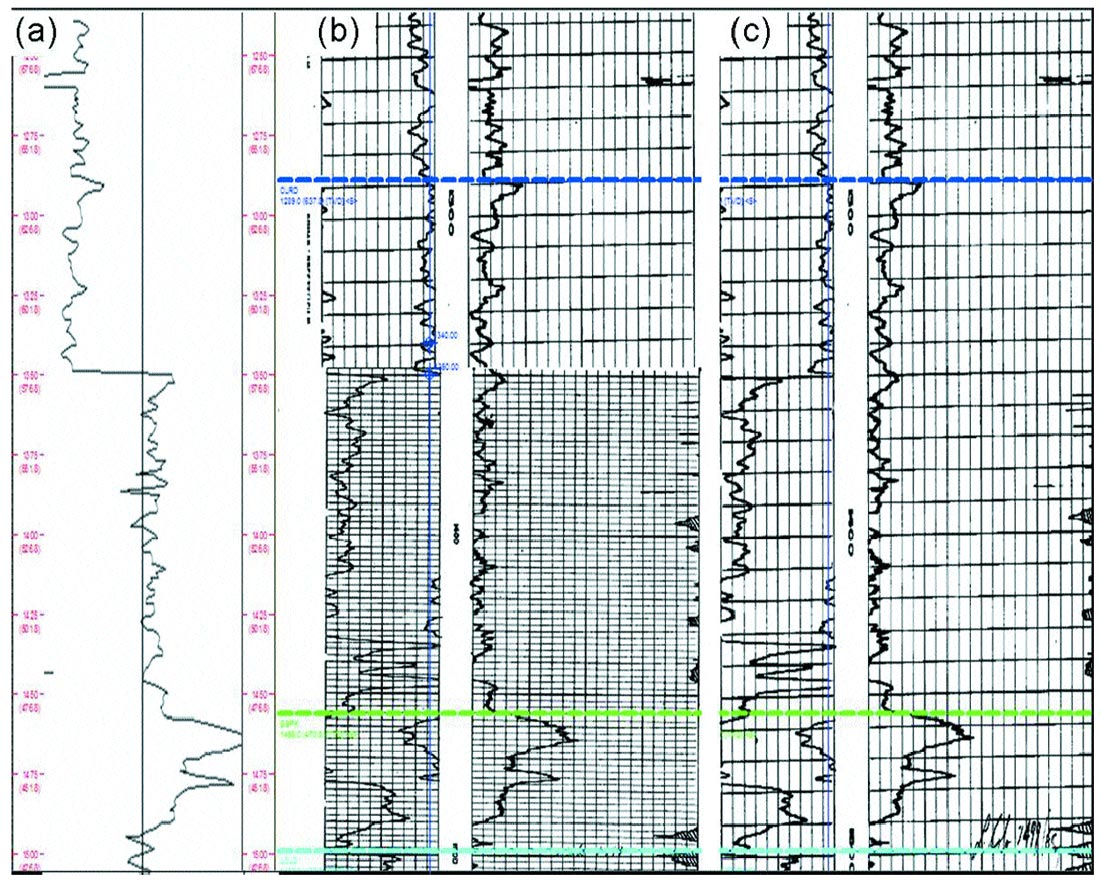
One common problem with older logs, is that they have often been digitized from paper and from time to time human error enters the equation. Figure 3a shows a dramatic acoustic velocity increase at 1350m. Referring to the raster copies of the logs (Figure 3b), we see that there is a change in the grid at the velocity break suggesting that there may be a digitizing problem. It is possible that the digitizer thought that this was the location of a scale change although we note that more often scale changes are missed rather than inserted by mistake. To check, we can often electronically peel back the lower log to see the overlap zone as shown in Figure 3c. While this is easy to check and to fix once recognized, we must visually recognize the possible error, making it potentially harder to diagnose.
Sonic logs are effectively the result of geophysical processing being applied to an acoustic measurement of the subsurface (similar to first-break picking), which can have the same problems as surface seismic data in terms of noise, tool problems, etc. An example is presented in Figure 4a, where erroneous values in the sonic log have made it all but useless for synthetic generation. When we look at the repeat log (Figure 4b) we see that the same erroneous values occur but not always at the same depths. This does not mean, however, that the data itself is poor, but perhaps has not been fully QC’d.
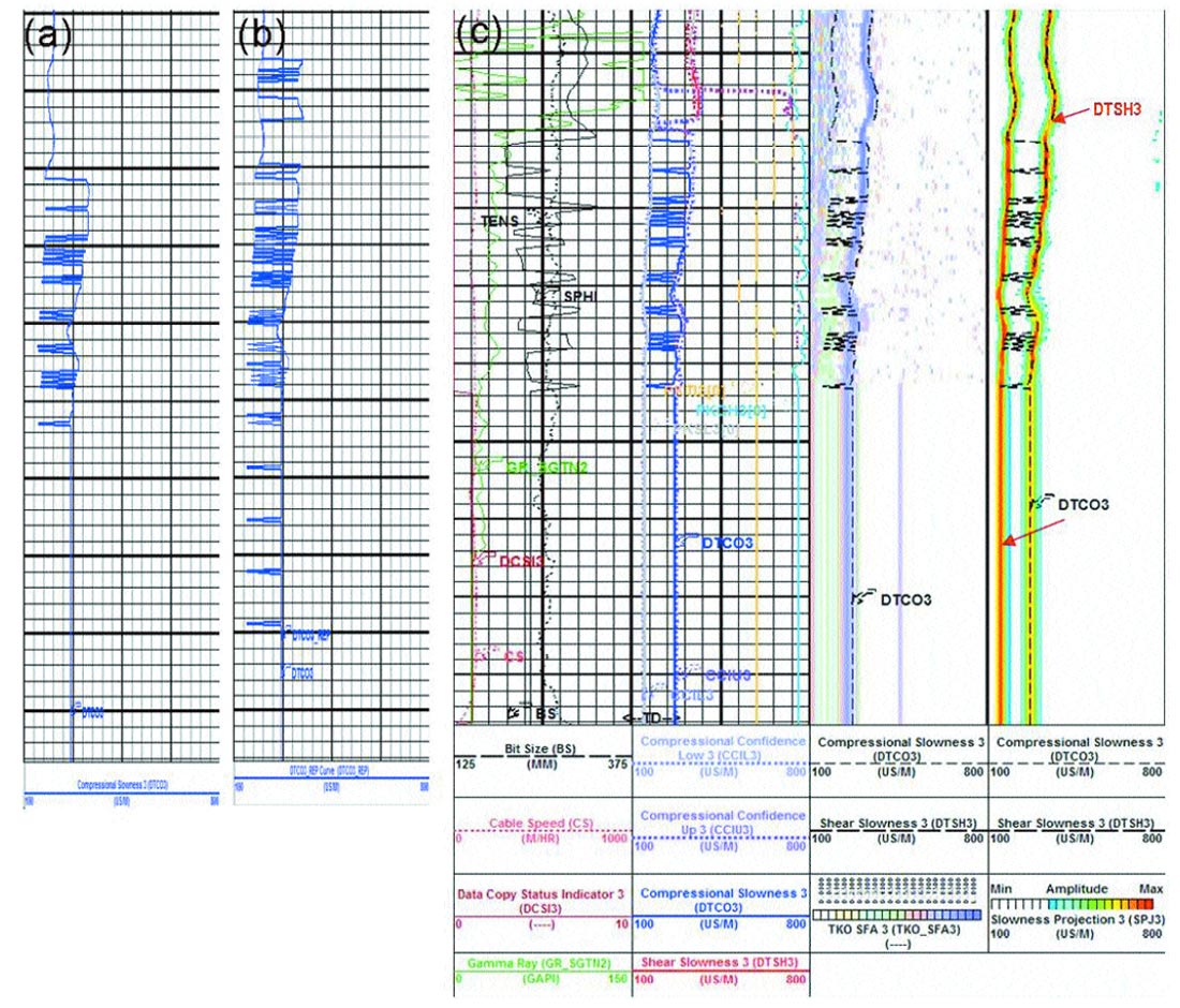
Looking at the full waveform presented in Figure 4c, we can see that the semblance autopicker has jumped from the compressional waveform (DTCO3) to the shear waveform (DTSH3). The human eye quickly observes the error in the computer semblance pick – so, like seismic, we should be QC’ing the processing of well log data. It is also a good idea to request and archive a copy of the raw waveforms from your logging company so that the processing can be revisited as new technology becomes available.
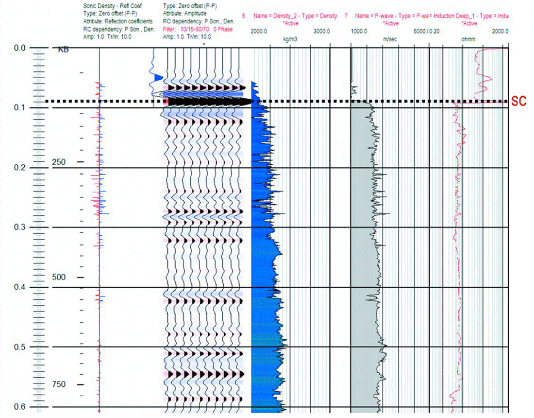
Another common pitfall often encountered by junior geophysicists is the “casing point reflection”. Logging runs typically extend from TD up to surface casing but should be truncated at the casing point before being interpreted. As we record up the borehole from relatively slow velocity shallow formation into solid steel casing, there is a large impedance contrast that manifests itself as a high amplitude event on the synthetic (Figure 5), which is solely associated with the surface casing (SC) not geology. This is easily spotted if all the logs are inspected in conjunction with the density and sonic, and we are aware of our location in the borehole. The resistivity tool shows a large increase when entering casing and provides a useful QC in this case. There are instances where this phantom event has been interpreted as a shallow marker and used to correlate across townships of data, despite not being a real geologic marker. Although this may seem to be an easy pitfall to avoid, it is far more hazardous when we consider all the intermediate casing points in deep boreholes.
We believe that the examples presented above highlight the necessity for interpreters to pay close attention to the well logs, to the point of having a general understanding of the data acquisition and processing and an idea of the borehole conditions. If in doubt, logs should be QC’d by a petrophysicist.
The order of operations
Thankfully, good logging runs without washouts or processing problems do occur, but that is not all that we are concerned about. When correlating logs to seismic, we know that we are calculating a synthetic from flawed log data and correlating it to flawed seismic data, but how often do we consider the effect of our choice of software. After all, most of the software in use by major E & P companies has certainly undergone rigorous testing, right? True, but that does not mean it is perfect. The software may be running on a flawless computer but programs often do not always work the way we expect or assume.
Figure 1 shows the processing flow used by many software companies to create synthetics, however, are they all the same and, if not, does it matter? A comparison of the order of operations used by several of the major software vendors (Table 1) shows that not every package contains the same order of operations – and it matters.
| Flow A | Flow B |
|---|---|
| Table 1. Comparison of flows for creating synthetic seismograms | |
| Load logs (sonic & density) | Load logs (sonic & density) |
| Calculate impedance | Calculate impedance |
| Calculate reflectivity | Convert to time |
| Convert to time | Calculate reflectivity |
| Convolve with wavelet | Convolve with wavelet |
The only difference is the order of steps 3 & 4, but does it matter? Three different synthetic seismograms created with identical well logs and wavelets (Figure 6) should theoretically be identical, however we observe that the first two traces are reasonably similar but the third trace, the one that uses flow B, is quite different. The only difference is the software used to create the trace.
Does the wavelet make a huge difference?
Let’s assume that the log data is perfect and the software is creating synthetics as we expect – let’s consider the wavelet. Often the first thing an interpreter does with his or her seismic data upon receiving it from the processor is to correlate it with a synthetic, and, in those first few minutes, several judgments about the quality of the data and the seismic processing are made. The wavelet is a critical factor when generating the synthetic but does it matter which one we use? The answer depends on what we are doing with the synthetic. For example, if we are simply estimating the approximate phase of the data (within 45°) and identifying the zone of interest, then most wavelets will be fine, generally. If however we are working on a more detailed analysis, for Q-estimation or impedance inversion, then the wavelet can critically influence the result.
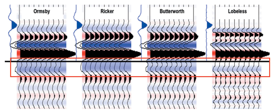
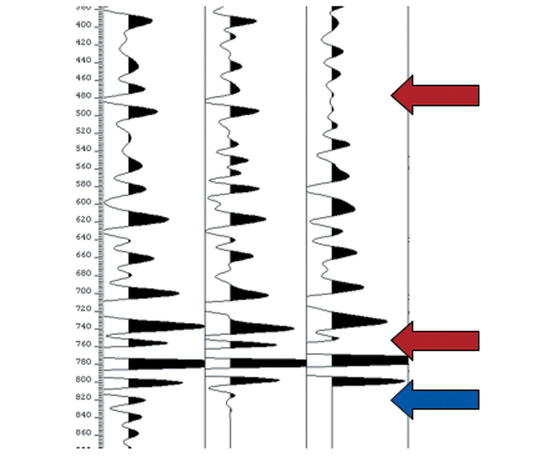
A comparison of a strong reflectivity contrast with four different wavelets is shown in Figure 7. While the main event does not vary much in this example, many of our hydrocarbon targets are contained in the side-lobe of a major event (e.g. Wabamun porosity, Slave Point, Lower Mannville sands, etc.). The frequency content of the wavelet should closely match the wavelet contained within your seismic data, the estimation of which is another paper in itself.
Making a synthetic tie
We’re happy with our input logs, the synthetics are being generated as expected and the wavelet is appropriate for our seismic tie – so let’s tie the synthetic to the seismic. Most likely all interpreters have had some ‘fun’ tying synthetics to seismic data, so we are just going to illustrate one of the more bizarre software glitches.
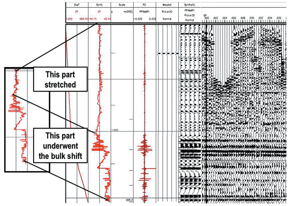
In our last example, applying a bulk shift to a synthetic within a commercial software program went awry (Figure 8). A standard script was run to apply a specified time shift. What resulted, however, was that instead of applying the bulk shift, the program applied a stretch to the first portion of the log, and a bulk shift to the rest, resulting in a well log that appears significantly longer than it is in reality. We note that the synthetic looks reasonable in that upper portion that was stretched and we can even convince ourselves that the tie is reasonable as the seismic is low fold in the shallow section so not all the events are correctly represented. But these events are not real! It is important to keep an eye on your time-depth curve and don’t take your software for granted.
Final comments and key points
We have presented a series of examples in which the creation and use of synthetic seismograms have created issues for interpreters. Synthetic seismograms are not as simple as they seem and many things can go wrong, so we advise:
- Use all available logs for QC
- If in doubt, check the paper logs
- Just like seismic, QC every step of well log processing
- If you need help, call your petrophysicist
- Know the borehole environment
- Keep an eye on your time-depth curve
- Know your wavelet
- Not all software is created equally
Not discussed but just as important are other more complex factors, such as sample rates during depth-to-time conversion, AVO effects, attenuation and imaging effects. All these factors, and others, are contained within the seismic data we are correlating or our 1D simple synthetics, which can also lead to erroneous conclusions.

Acknowledgements
We are grateful to Apache Canada Corp. and Nexen Inc. for permission to present this material at the CSEG lunchbox talk in April, 2008. Additionally, we thank the audience at our lunchbox talk for participating in a lively discussion, providing personal experiences and asking interesting questions. Additionally, we would like to thank Dave Monk, Marco Perez and Ron Larson for their critiques of this article. We would be remiss if we did not acknowledge the support of our spouses, Ian Crawford & Elizabeth Anderson, in putting up with us while we pulled out our hair in trying to understand the issues around what most of us take for granted.
The Schlumberger Oilfield Glossary can be found at: http://glossary.oilfield.slb.com/


Join the Conversation
Interested in starting, or contributing to a conversation about an article or issue of the RECORDER? Join our CSEG LinkedIn Group.
Share This Article