Sonic Velocities and Depth Conversion

The current method(s) of converting seismic time data to depth are methods created to work-around the lack of access to an adequate volume of velocity data.

Access to sonic velocities provides the opportunity to move all variables of the depth equation into the depth domain where mathematically and geologically correct depth maps become a reality.

Sonic velocities are applicable in the process of converting seismic time data to depth under the following conditions:

• The sonic logging tool is intrinsically unaware of geology.
• Geophysical depth maps are computer driven depth maps.
• Seismic time data integrated into the depth domain.
• Geological depth models created in accordance with local and regional geology.
• Contrived geologic depth model imposed on the geophysical depth map.
• Validation by integrated velocity map compared to geologic depth model.

The intervention of a geologically contrived depth model (includes all wells deviated and vertical) merged with the geophysical depth map produces a depth map that is mathematically and geologically correct (to the extent provided by available data).

The integration process ties seismic traces located at each well in the seismic data patch.

Integration of the interpreted seismic data into the depth domain gives rise to a geophysical depth map, in the depth domain. A geologically contrived depth model integrated into the geophysical depth map. A valid integrated velocity map emulates the geological depth model.

Introduction

This objective of this paper is to illustrate the value of extracting and applying velocity information from sonic digital data. From a theoretical standpoint, the continuous sonic should be the best, and most, complete form of velocity information possible to obtain at a given location. Lindseth, (1982). The recorded sonic log trace is a permanent record of a measurement recorded by a mechanical tool that is intrinsically unaware of geology. The recorded value is simply a value that fulfills the requirements of the depth equation.

A segmented sonic log curve records an interval transit time across each segment, regardless of segment size. The inverse of interval transit time is velocity. Interval transit times, when grouped on an interformational basis, provide information regarding interval velocities and/or average interval velocities over groups of log segments. There are no other logging systems capable of providing such information in such detail. Sonic log velocity detail, when collated, processed and applied, is a key critical factor in the production of depth maps that are mathematically and geologically correct. Sonic velocities provide a viable link between the interpretational role of geophysics and the observational role of geology. This is an underutilized data source that cannot, and should not, be bypassed in favor of any other source of velocity.

The introduction of the sonic logging tool to the petroleum exploration community occurred in the early to mid 1950s. Direct extraction of velocity data from well logs soon proved unreliable as a source of velocity data used in the process of converting seismic time data to depth data.

The introduction of computers and contour mapping software in the mid-1980s theoretically made the timely presentation of accurate depth maps to exploration management a reality.

The depth conversion process outlined in this paper takes the following steps.

1. Define well data and seismic data in terms of distinct domains; depth and time, respectively.
2. Extract velocity data from digitized well logs in LAS format.
3. Edit the sonic digits for null values approaching zero.
4. Sample the continuous curve at constant depth increments. Each increment provides an interval transit time across the sample increment.
5. Integrate seismic data into the depth domain in order to maintain the mathematical integrity of the depth equation.
6. Create geophysical depth maps in the depth domain applying integrated seismic time and sonic velocity.
7. Merge geology and geophysics by integrating a geologically defined depth model into the geophysically derived depth map.
8. Generate an integrated velocity map, integrated seismic time map in support of the imposed geologic depth model.

As this paper will show, the problem lies not with the sonic tool or the data that it records. The problem lies with the philosophy within which the data is applied. To quote A.R. Brown, (1992), “The most pressing need today is to make proper use of what we already have”. This paper presents a method that makes appropriate use of two sources of mathematically correct velocity data.

Sonic velocities are interchangeable with check-shot velocities in any of the processes discussed in this paper, as sonic and check-shot velocities fulfill the mathematical requirements of the depth equation. Both tools, being intrinsically unaware of the recording environment, produce different velocities because both tools are distinctly different tools. The only similarity is that the recorded data fulfills the mathematical requirements of the depth equation. Signal purity is considered immaterial.

The Depth Domain

The depth domain is the repository of all data measured in vertical units of distance, such as, formation tops, sonic and check-shot velocities, conceptual geologic models etcetera.

In the depth domain:

1. The only valid seismic traces are those traces that tie well data in the depth domain.
2. The opportunity for geologic intervention with a geologic depth model, based upon observational criteria, is possible. (Shultz (1998) describes a 3D seismic data set that contains 11.5 million traces and 11 wells. A geologic cross section that links the 11 wells will provide no inter-well geologic details. Of the 11.5 million seismic traces the only valid seismic traces are the traces that, when integrated with the depth domain data in the depth domain, directly tie the 11 wells.
3. A conceptual geological depth model, created from observational inputs, when imposed on the computer-generated depth map that is mathematically correct, produces a geologically correct depth map. This procedure merges the geological and geophysical disciplines.

The Time Domain

The time domain is the repository of all data measured in vertical units of time. As time domain data are intrinsically unaware of geology, consider:

1. The creation of depth maps requires variables in time and velocity. Seismic velocities derived from seismic data are dependent upon the seismic data interpretation. Subsequent interpretational alterations have effect on the dependent velocity. The application of dependent vector velocities compromises subsequent processes.
2. Seismic stratigraphy is a geological procedure conducted in the time domain. Seismic stratigraphy is a method that determines the nature and geologic history of sedimentary rocks and their depositional environment from seismic evidence, Sheriff, (1980).

The Mathematics of the Depth Equation

All depth maps revolve around the depth equation: Depth equals Velocity multiplied by One-Way-Time: (D = V*T). Possessing components of magnitude and direction, Depth and Velocity are vector quantities; Time is a scalar quantity as its only component is magnitude.

Critical examination of the depth equation requires that the only stipulation on the velocity vector is that it be independent of the time variable. The depth equation does not discriminate between various geological properties.

Etris et al (2001), states that seismic velocities are not right for true depth conversion. In paragraph two, they list what the deliverables of a depth conversion project might be. Some of the requirements that Etris et al (2001) recognized as necessary were: seismic data volume in depth, data grid volumes from seismic and wells, a velocity model and an uncertainty analysis. Etris does not elaborate on how one might achieve a seismic data volume (2D or 3D) in depth.

Geological Processes in Contrast to Geophysical Processes

Two distinct processes contribute to the creation of a mathematically (uncompromised) and geologically correct (geologically contrived) depth map.

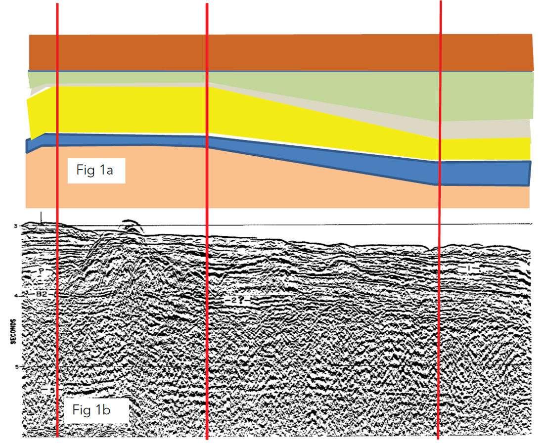
A geological process is an observational process that addresses all well data in the depth domain. Figure 1a presents a hypothetical geologic cross section where it is shown that when formations are linked from one well to another, there is no indication of intervening geology. Geologic cross sections are a depth domain process. Figure 1b presents a seismic section that, hypothetically, parallels the geologic cross section of Figure 1a. In units of vertical time and by interpretation, the seismic data of Figure 1b illustrates the interpretive geologic detail that the cross section of Figure 1a lacks. Integration of the information contained in Figures 1a and 1b, in the depth domain, is required to maintain the mathematical and technical integrity of the depth map.

The second process is a geophysical process that encompasses all of the computational manipulations required to create mathematically correct depth maps. The most important step in the process is the process of integrating seismic 2WT data into the well data of the depth domain. The penultimate step in the geophysical process is the generation of a geophysically generated depth map. A depth domain geophysical depth map that, in and of itself and being digital in origin, totally lacks geological connotation yet provides opportunity for geologic refinement of the geophysical depth model. This map provides an essential platform upon which geological intervention finalizes the final geological depth map. There is a point at which these two disciplines must merge in order to create a mathematically and geologically correct depth map.

Sonic & check-shot logging tools

Like all other logging tools, the sonic tool is intrinsically unaware of geology. The sonic logging tool, designed to record the travel time of an energy pulse emitted from a transmitter to a receiver located a fixed distance from the transmitter, measures interval transit times in units of time per unit distance, the inverse of which is velocity.

Table 1 illustrates the superior attributes of the depth conversion process that utilizes sonic derived velocities by direct comparison of the) process that converts seismic time to depth utilizing seismic derived velocities. The check-shot system operates similarly but with coarser intervals.

TABLE

Gretener, (1961), Herron, (2014) and other authors have attempted to compare data recorded by the sonic and check-shot tools. The sonic tool and the check-shot tool are two different tools that measure the interval transit times of different thicknesses of material and under differing environmental conditions. Being mechanical, these tools are intrinsically unaware of geology because such tools, for reasons of design, cannot interpret the nature of the recording environment.

The check-shot survey records interval transit times at comparatively coarse intervals, whereas, the sonic tool provides a continuous record measured across comparatively much shorter intervals. Hypothetically, the sonic log, by virtue of its ability to provide a continuous record, is significantly more valuable than the check-shot survey as a source of independent vector velocity.

The sonic log display is a continuous curve which, when segmented into discrete intervals, yields a continuous record of interval transit time, average interval transit time, interval velocity and average velocity.

Gretener, (1961) compared the noticeable time discrepancies between the sonic log and check-shot survey recorded in a number of wells in Alberta, Canada, with the intent of discontinuing the use of the check-shot survey. Gretener (1961) concluded that the time deviations between the two tools were systematic and independent of velocity and lithology (sic geology).

This paper expands on the conclusions of Gretener (1961). Systematic and independent of geologic velocity and lithology, suggests that reassessment of the data recording and application methods of time and depth domain data is required. This paper elaborates on the results of such reassessment.

Herron (2014) attempted to calibrate the sonic tool results with velocities recorded by the check-shot tool by “blocking” the sonic log data at recognizable boundaries. This procedure is tantamount to altering recorded data to fit a preconceived conclusion; that being, the check-shot survey was correct and the sonic data required alterations. Insofar that both tools are mechanical instruments and do record data in similar environments, does not infer that both tools were aware of the recording environment in terms of geology. These tools do not possess the observational prowess of the human brain and therefore record what they measure.

Conventional depth conversion

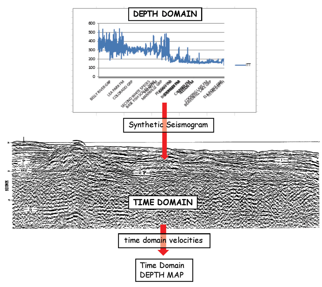
As shown in Figure 2, the conventional depth conversion process, herein defined as any conversion process that does not integrate seismic data into the depth domain, relies on the integration of well data into the time domain as opposed to integration of time domain data into the depth domain. Integration of well data into the seismic data involves the creation of a synthetic seismogram from raw sonic log data (density log data are applied as availability allows), and the calculation of reflection coefficients in units of vertical time. The reflection coefficients, when plotted, form a reflectivity spike series, which, when convolved with a wavelet of known characteristics, produces a synthetic seismic trace in units of vertical time. The synthetic seismogram is the agent that integrates well data into the seismic data.

For reasons of replacement velocity discrepancies, integration of the geologic information into the seismic data involves a “best fit” process that associates amplitude events identified on the synthetic trace with similar amplitude events on the seismic reflection trace.

Data processing replacement velocity is an arbitrary choice that dictates the two-way-time position of the seismic data, within the seismic section graph space. A replacement velocity using the shallowest last sonic recording depth and the data processing datum provides a means of calculating a replacement velocity based on well data. When data processing and sonic replacement velocities are equal, the two-way-time location of the shallowest sonic recording allows transfer directly to the seismic data. Hypothetically, the transfer of formation tops from well to seismic data should then be resolvable by mathematical means.

As history demonstrates, the conventional depth conversion (conventional, as in the procedure promoted by geophysical interpretation software vendors, where seismic data is the source of velocity data) method arose from an initial absence of adequate volumes of vector velocity data.

A most critical compromise occurred when workers, under the perception that the sonic was actually recording geological interval transit times, forced geologic connotation on the sonic logging tool, an instrument that is intrinsically unaware of the geological environment in which it was recording. In the absence of an integration procedure that brought all variables into the depth domain, the resultant conclusion was that sonic velocities were unusable for depth conversion purposes. Access to sonic derived velocity data and appropriate data management methods resolve all such compromises.

Denham et al (2011) cited sonic logs, or check-shot surveys, as the prime source of velocity. In the absence of check-shot or sonic velocities Denham et al concisely discusses the various methods of the conventional depth conversion processes that involve various sources of velocity, all in the time domain. Denham et al provides a suite of maps that demonstrate the effect of a variety of time domain sourced velocities on the final depth map. Denham et al does not mention the potential of integrating seismic time with well data, in the depth domain.

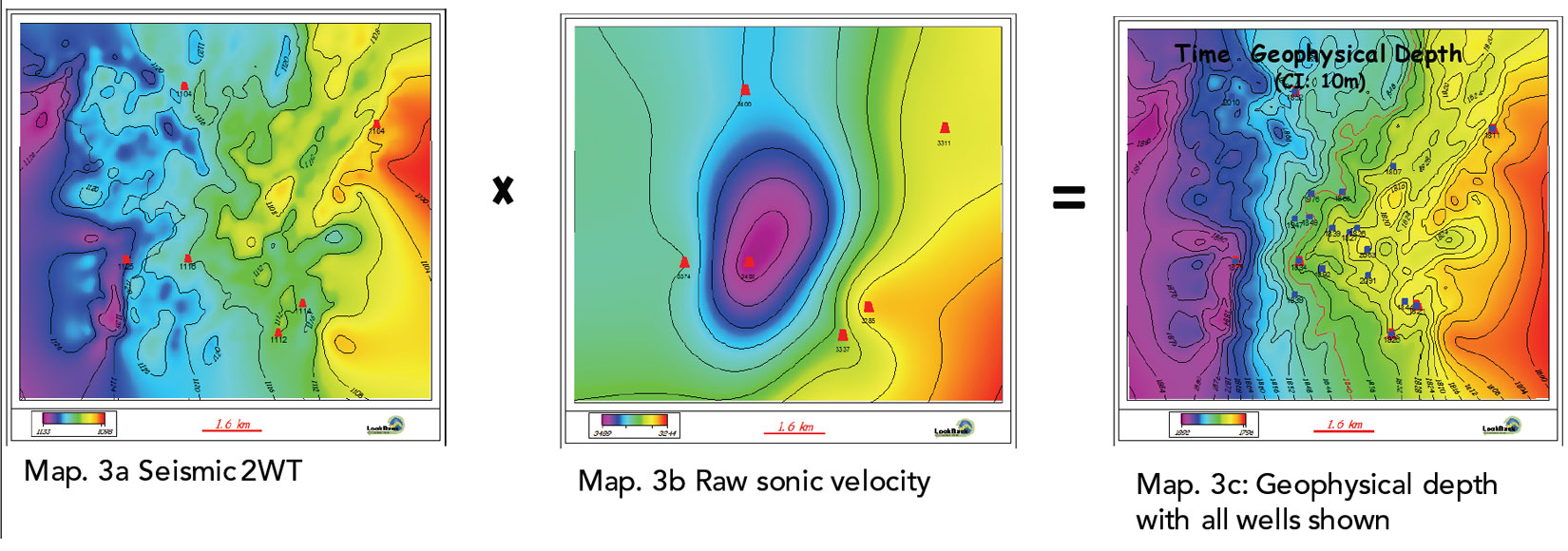
The map suite shown in Figure 3 illustrates the process that leads to failure more often than not. The seismic data of Map 3a multiplied by the raw sonic velocities of Map 3b produces the geophysical depth map of Map 3c, in the time domain. In the absence of an integration process, map generation can only occur in the time domain. The worker is unintentionally bound by the quality of the seismic data involved.

Unconventional Depth Conversion

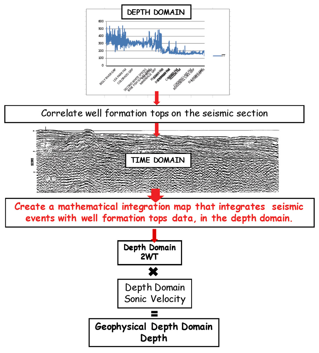
The unconventional depth conversion method, shown in Figure 3, involves velocity data extracted from processed, or raw, sonic log digital data or velocities extracted from check- shot surveys, the integration of time domain data into the depth domain and the inclusion of a geologically contrived depth model. The maps of Figure 4 suggest merging the highly detailed seismic time data with scantily spaced time data of the sonic log.

The data integration process is a key step in applying sonic log (or check-shot) velocities to the depth conversion procedure. Integration of seismic time into the depth domain involves the interpreted time domain data and a process that ties time domain data to depth domain data, as indicated by the workflow of Figure 3. Integration requires a map that converts time domain data to time data, in the depth domain for each formation of interest listed in the well spreadsheet.

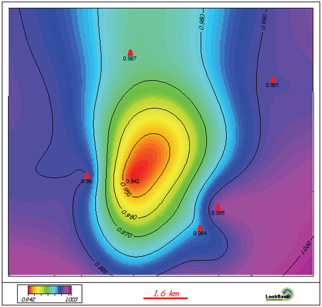
The integration map (Figure 5) is a dimensionless map of the ratios derived from dividing depth domain (sonic) 2WT by interpreted time domain (seismic) 2WT at each well location in the seismic patch. This has the effect of rendering only those seismic traces at each well as the only valid depth domain time traces. Multiplication of the time domain (seismic) map by the integration ratio map produces an integrated time map in the depth domain (Map 9b of Figure 9).

Theoretically, on the assumption that formation contamination can only increase interval transit time a logical presumption that the seismic tool records seismic data whose travel path is consistently through uncontaminated rock would have a lower interval transit time through the same rock interval as sonic log measurements recorded in contaminated rock exists. It follows that the calculated ratios should be unity or greater. The integration map of Figure 5 presents values that are less than unity. The reason for this discrepancy is that the seismic data has not been properly located in the time versus distance graph space. (The current data processing selection of replacement velocities is an arbitrary choice. A calculation involving the depth to the shallowest sonic reading, in conjunction with the seismic reference datum mathematically provides an accurate replacement velocity at each well. Note: It is not the intention of this paper to elaborate on the appropriate placement of seismic data in the time versus distance graph space.

Sonic log and data processing data can provide the required information in this regard.)

In 1991, Dr. Phil Schultz moderated a meeting of top geo-scientists from several major exploration and service companies that discussed methods of integrating borehole data and seismic data. The major topic being seismic imaging, to which one member contributed the impression that integration involved moving borehole measurements into the spatial picture constructed from seismic data. The member added that this tie was easy in vertical wells but difficult, if not impossible, in deviated wells.

Later in the discussion, the same member added that sonic velocities were the most important parameter in tying log data to surface data as it allows switching back and forth between time and depth domains. Conversely, this paper shows that sonic velocities allow the integration of the spatial picture constructed from seismic data into the spatial picture constructed by the borehole measurements in the depth domain, a process that ties vertical and deviated wells to well data with ease.

In respect of any seismic time data set, the only valid depth domain seismic traces are the traces that correlate with wells within the depth domain. Schultz (1998) discusses the process of creating a velocity model from 11.5 million seismic traces and 11 wells, implying that all of the seismic traces are valid, in the time domain. In the depth domain, the seismic traces that tie the 11 wells are the only valid traces. The remainder are considered to be contour options.

Sonic Log Processing

All processing procedures occur in a spreadsheet environment.

Sonic log data, recorded in vertical boreholes, is a valid input to a mathematically correct depth conversion method. Sonic data recorded in deviated boreholes are not candidates for direct depth conversion because, for directional reasons, deviation requires redefinition of the velocity vector. However; such wells do have an associated true vertical depth (TVD) and therefore, incorporation of such data in the final geological depth map is essential.

Log data processing involves:

• Edit for null values and values approaching zero.
• Neutralize the effects of tool travel speed and borehole conditions on the recorded interval transit times (as effects due to travel speed and borehole conditions can occur simultaneously, such effects cannot individually be corrected, neutralization is the only option).
• Calculate velocity (replacement) and 2WT from the seismic reference data (SRD) to the shallowest sonic log recording.

The processing routine, developed and copyrighted by LookBack Exploration Ltd accomplishes these requirements. Log processing results are unique to every well.

In the spreadsheet, processing causes apparent minor changes to interval transit times and hence interval velocities. At map scale, the differences between processed and raw log data, becomes obvious, as illustrated in Case History 3.

Ideally, sonic log recording occurs from total depth to near ground level. Every geologic formation should be (but rarely is) identified on the log. Inclusion of additional geologic formations in the spreadsheet as required is possible.

Well control and safety require cemented surface casing from near ground level to a depth equal to or deeper than 10% of the predicted total depth. The last (shallowest) sonic reading should occur within close proximity to the surface casing shoe.

Geological Intervention

Geologic intervention is the process that integrates geological and geophysical disciplines and produces a geologically and geophysically competent velocity model in the depth domain.

The imposition of a contoured conceptual geological depth model that includes all wells (vertical and deviated) in the seismic data patch in contour map form, on a geophysical depth map requires rearrangement of the geophysical depth contours to accommodate the conceptual depth model. The resultant contour map is a mathematically and geologically correct depth map, in the depth domain.

Validation of the geological depth map involves division of the geological depth map by the integrated time map to produce a geological velocity map. Shape similarity of the geological velocity map to the geological depth model provides validity of the geological depth model. If the resultant velocity map is valid, the geologic depth model is valid.

In the event of invalid velocity contours (lacking geologic support), the geologic depth model must be redrawn and imposed on the geophysical depth map to eliminate such anomalies, will eventually result in a valid geological velocity map. Additional drilling will determine the validity of the imposed geological depth model.

In the introduction to his one-day short course on velocity model building, Shultz, (1998) writes, “ . . . processes like depth migration and depth conversion of 3D seismic data require a geologically and geophysically competent velocity model”. Sonic velocities provide for the creation of a geologically and geophysically competent velocity model by merging a geophysically derived time in the depth domain with a valid geologic depth model.

The case histories included in this paper will show that the creation of a competent velocity model evolves from seismic data (2D or 3D) integrated with a geological depth model that was created by a human brain. The human brain is the only readily available instrument that possesses observational capability and the ability to visualize a competent depth model.

The case histories demonstrate that integration of time domain data with depth domain data, in the depth domain, provides a method of incorporating deviated wells.

Case Histories

Case History 1:

This case history consists of average velocity maps that cover a generous portion of the south-central plains area of Alberta, Canada. The map of Figure 6 shows average sonic velocity from a constant seismic reference datum to the top of the Nisku Formation. Figure 7 is a depth map from the same wells referenced in Figure 6. Comparison of the velocity and well depth maps of Figures 6 and 7 respectively, demonstrates that the regional velocity model does have striking resemblance to a regional depth map drawn from the same data.

Similarity of the mapped depth and velocity occurs because average velocity and depth have the same start and endpoints. Both maps, involve over 2600 processed sonic logs.

Case History 2:

The data for this case history consisted of an interpreted 3D seismic survey in the form of seismic two-way-time picks and their corresponding geodetic coordinates. The geologic horizons interpreted by the donor are, the Devonian Age Winterburn and Woodbend Groups. The basis of this case history involves a suite of maps that cover an assumed depleted Devonian oil field in south central Alberta, Canada. Processing has neutralized the effects of borehole conditions and tool travel speed. Only the Winterburn/Nisku work will be discussed, a result of space limitations.

There are twenty (20) wells located within the 3-D data patch on the base map of Figure 8. Of the twenty (20) wells, Six (6) wells are vertical with sonic logs recorded from total depth to near base surface casing. The basis of the final geophysical depth map includes only these six (6) wells. The remaining fourteen (14) wells are deviated and cannot be included in the geophysical depth conversion process because significant deviation of the well bore from the vertical requires redefinition of the velocity vector. Nonetheless, deviated wells have a true vertical depth to formation and must be included in the final geological depth map.

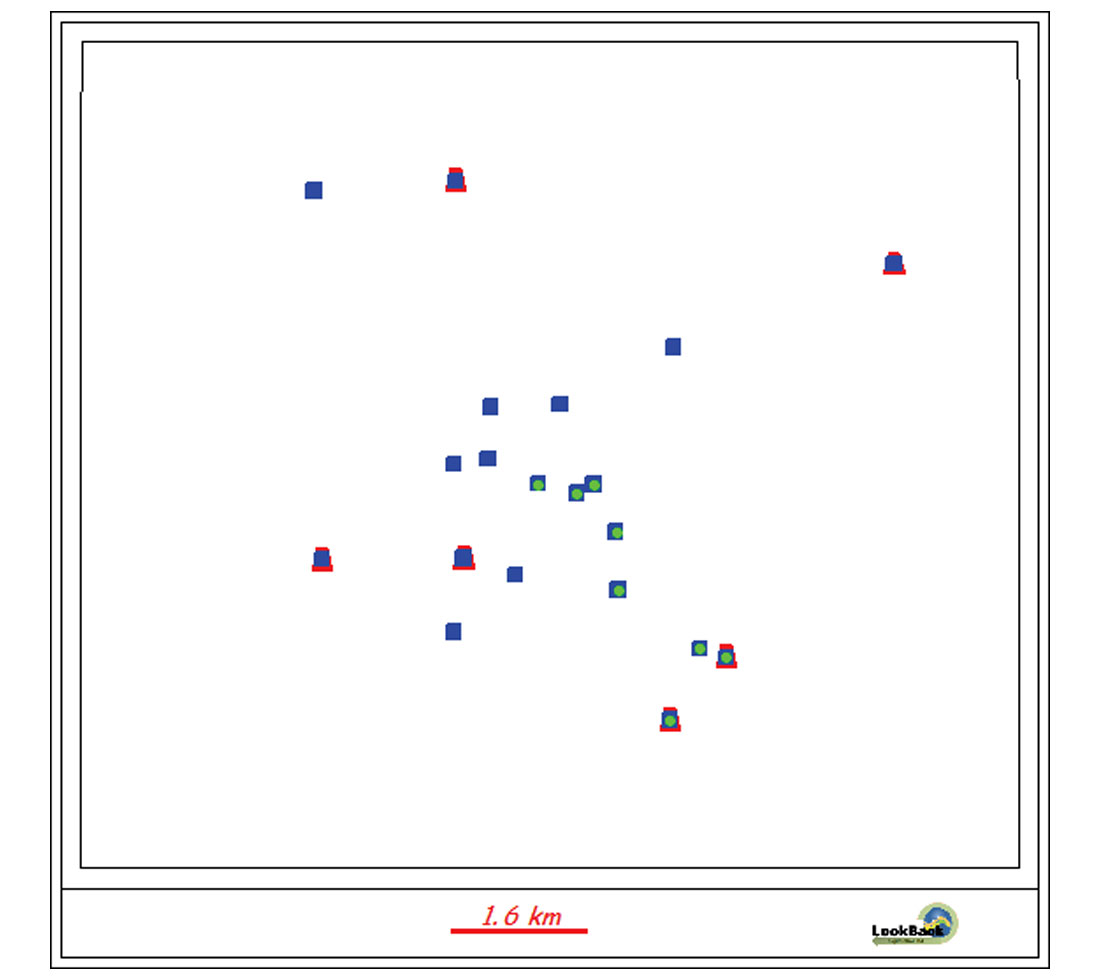
Conversion of true vertical depth elevations of all deviated wells to a common reference datum, ensures that all 20 wells are included in the final geological depth map. In order to ensure the final depth map is mathematically and geologically correct, geology must intervene with a depth model that includes all twenty (20) wells.

Integration of Time Domain Data into the Depth Domain

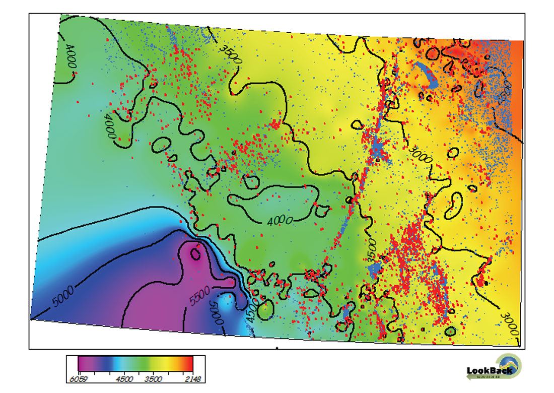
The integration process gathers all of the variables of the depth equation into the depth domain. The maps of Figure 9 illustrate the result of merging the seismic time domain data with the depth domain data. This unites all of the depth equation variables in the depth domain where base data is fixed. Figure 9b becomes the time map to the final geophysical and geological depth map.

The sequence of maps in Figure 10 (Map 3a, Map 9b, Fig 5, Maps 10a, and 10b), illustrates the integration process from time domain data to a geophysical depth map. The geophysical depth map accommodates only the six (6) wells that have vertical sonic logs and valid time domain traces. Integration effectively redraws the time domain map (Map 3a) such that the time traces, at each well, tie the well two-way-time precisely. Due to the lack of inter-well depth and velocity data, the placement of inter-well contours is due to computer mapping algorithms rather than by geology.

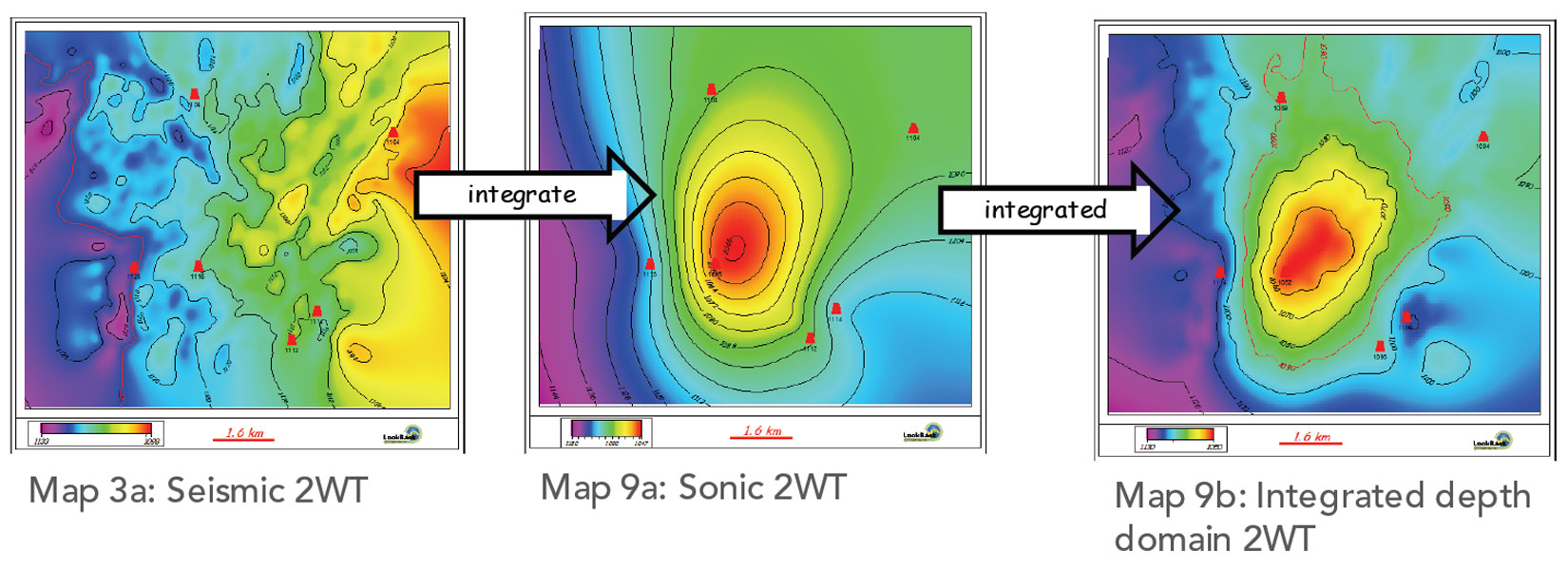
The process flows as follows:

1. Create the integration ratios map (Fig 5).
2. \Time domain time map (Fig 3a), times the integration ratio map (Fig 5) equals an integrated time map (Map 9b).
3. Integrated depth domain time map (Map 9b) multiplied by the depth domain velocity (map 10a) equals depth domain geophysical depth map (Map 10b).

Note that the geophysical depth map (Map 10b) is the result of geophysical/digital processes and is mathematically correct, but not geologically correct. The map is not geologically correct because all twenty (20) wells cannot be accommodated in the time domain by geophysical processes alone.

The only wells that can be accommodated in the digital domain are the six (6) vertical wells shown in Figure 8 because these are the only wells to which valid time domain values can be tied. However; Figure 8 includes 14 deviated wells that have a true vertical depth. Geology must intervene with a depth model that accommodates all of the wells that have associated valid vertical depths.

Geological Intervention

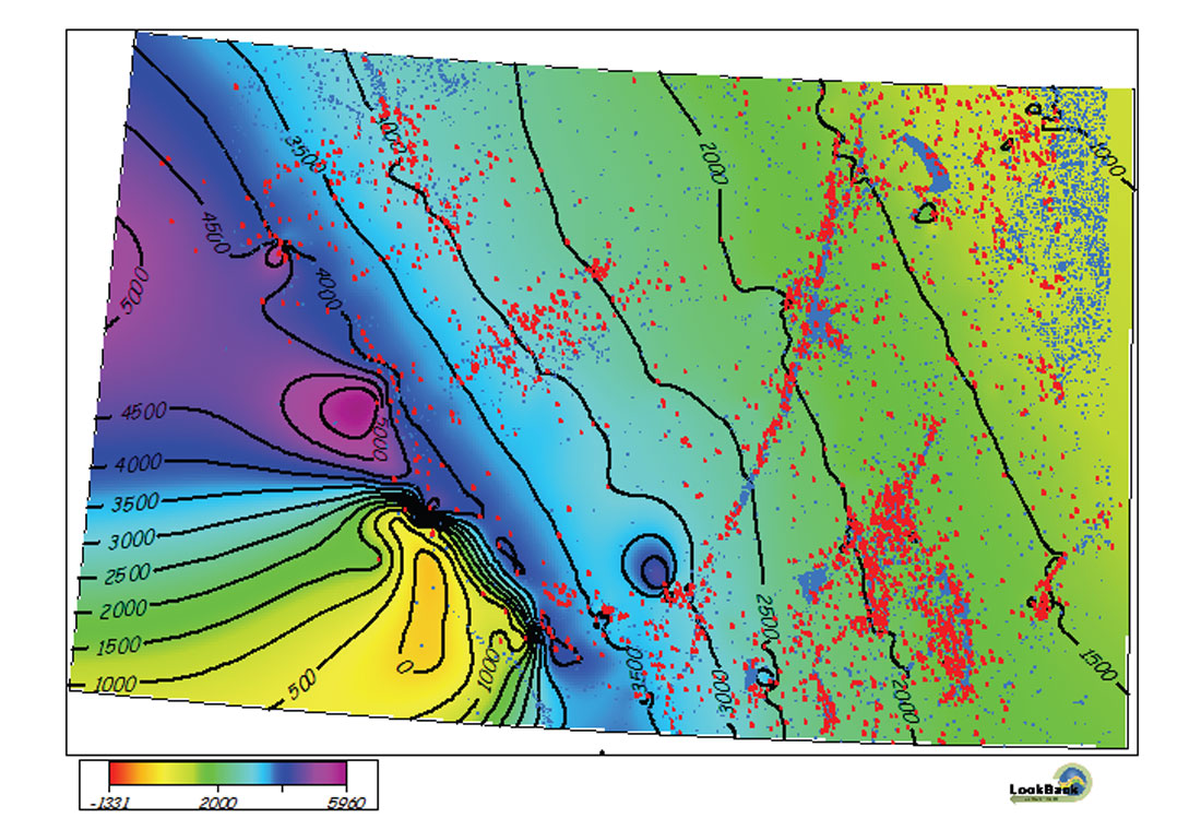
Geologic intervention is the final critical step in the depth conversion process. Figure 11 presents the final geophysical depth map with all twenty (20) wells located within it. Note that only six (6) wells are contour tied. The remaining fourteen (14) wells are not contour tied. In order to include all twenty (20) wells in the final geological depth map, a conceptualized, contoured geological depth model imposed on the geophysical depth map of Figure 11a. On the premise that all contours drawn between fixed data points are essentially contour options, the depth contours may be redrawn as the geologist sees fit so long as contour values at fixed well data points are honored.

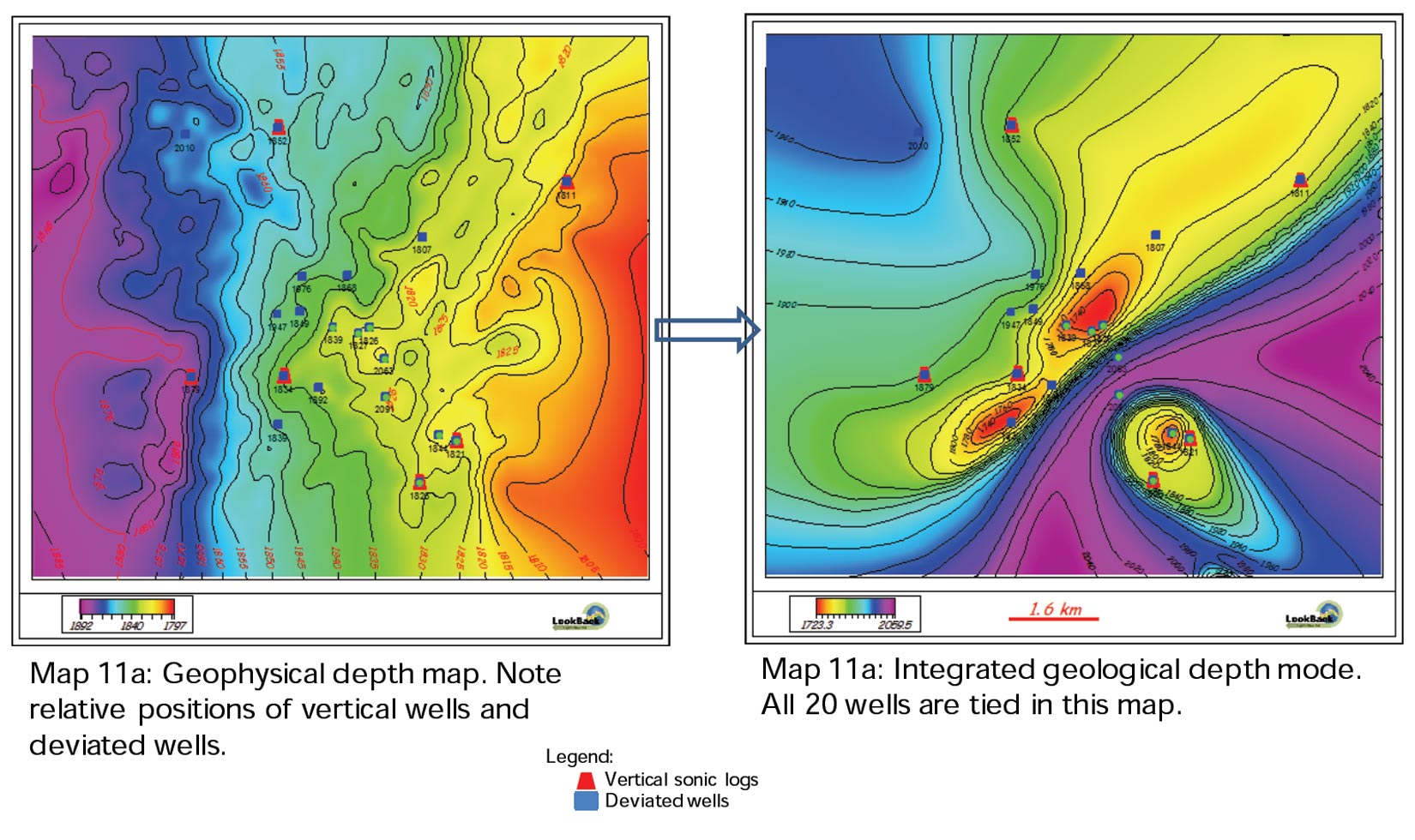
An added provision is that the final geological model must harmonize with the surrounding regional and local geology. This includes honoring the sedimentary and tectonic characteristics of the featured drilling target. An imposed depth model is shown as Map 11a, with all wells posted. Note that the contours tie all of the wells.

The validity of the depth model can be tested by dividing the geological depth model map (Map 11a) by the integrated depth domain time map (Map 9b) to create a new velocity map as shown in Figure 12.

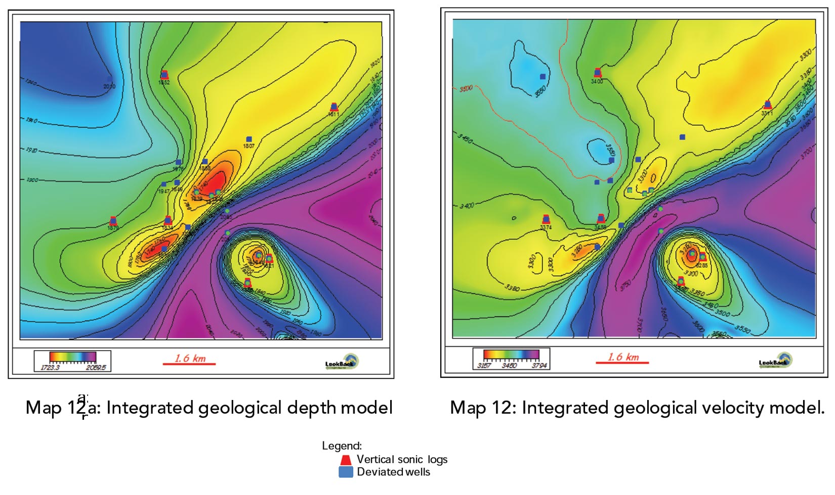
By comparison, the velocity model of Map 12 compares favorably with the geologic model in terms of shape. The geological depth model (Map 11a) was drawn to ensure that all of the wells were accommodated in the geological depth model and may not be the most accurate selection. It remains at the discretion of the geologist to determine the most appropriate model to apply.

Case History 3:

This case history compares and contrasts depth maps created using three (3) independent vector velocities sources, being check-shot velocities, processed sonic log velocities and raw sonic log velocities. All anomalies are located within a known oil productive area.

This example (Figure 13) is proprietary and is included only to demonstrate that sonic velocities will produce reliable depth features when compared to check-shot velocities.

Figure 13 shows a depth map, in the depth domain, created from a 2D seismic survey and 11 vertical wells. In each of the 11 wells, sonic logs and check-shot surveys data recorded from TD to near surface casing are available. The depth conversion process as applied as follows:

1. Interpret the seismic data.
2. Process the sonic logs for borehole conditions and tool travel speed.
3. Prepare an integration ratio map.
4. Integrate time domain seismic data with the sonic or check-shot time data.
5. Prepare sonic and check-shot velocity maps.
6. Multiply the integrated time maps by the respective well velocities.
7. Prepare the sonic and check-shot related depth maps

The depth maps of item 7 (above) require minor geologic intervention.

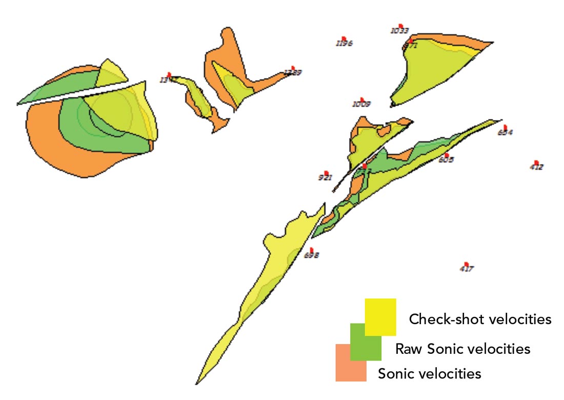
The map in Figure 13 consists of three layers as follows:

Layer 1: The top layer (yellow) shows depth anomalies created by applying check-shot velocities in the depth conversion process.

Layer 2: The middle layer (green) shows depth anomalies created by applying raw unprocessed sonic log data in the depth conversion process.

Layer 3: The bottom layer (orange) features depth anomalies created by applying processed sonic log data in the depth conversion process.

Of the eleven wells, one (1) well is a declared gas discovery, two (2) are oil discoveries and three (3) wells were plugged and abandoned with excellent oil indications. The remaining plugged and abandoned five (5) wells drilled two-way-time closures.

The colored anomalies of Figure 13 clearly show that processed sonic log data (orange) produces the most attractive drilling targets in all anomalies. Unprocessed sonic log depth maps suggest such data appears to outrank check-shot data in terms of attractive drilling targets.

Conventionally, the check-shot survey data is the velocity source of choice in this area. The seismic survey operator did not conceive of the necessity to integrate the time data with well data in the depth domain. Therefore, by assumption, all 11 wells drilled on seismic data controlled depth maps created in the time domain.

It is obvious that Figure 13 shows excellent agreement with check-shot derived contour maps. The fact that all three processes produce anomalies that overlie each other is further testimony to the fact that sonic velocity information are a reliable source of depth conversion velocity.

This case history also shows that the, final geophysical depth map, may well portray the most appropriate geologic depth models with little or no requirement for geologic intervention.

Conclusions

As demonstrated, compromising the mathematics of the depth equation causes a compromise of all further depth conversion processes. Failure to integrate interpretive data into fixed well data prevents geologic intervention and hence failure to merge geophysical effort with geological effort. Integration of time domain data into the depth domain is a most critical step in the depth conversion process because this step provides opportunity of the trained geological mind to intervene with a depth model that includes all wells.

1. Sonic log and check-shot velocity are the only sources of velocity that do not compromise the mathematics of the depth equation.
2. Access to, and management of, well log velocities makes the integration step possible.
3. Geology is intrinsically unaware of geophysics and vice versa.
4. All data collection and processing tools are intrinsically unaware of everything. Such instruments lack the observational capabilities of the trained geological mind.
5. Mathematically and geologically correct depth maps are possible via the integration of time domain data into depth domain data.

Acknowledgements

1. Dr. A. Easton Wren provided invaluable and much appreciated assistance in the preparation of this paper.
2. Shaunn W. Pickering provided specific sonic log processing expertise.
3. Dr. Fred Hilterman, Geokinetics, provided very useful construction comment in preparation of this paper.