Some Issues related to Seismic Imaging in Deep-Water Basins

Introduction

Obtaining high fidelity seismic images in deep water basins has several challenges. These run from the issues of dealing with noise to building accurate interval velocity models for Pre-Stack Depth Migration (PreSDM). Exploration, and development, in such basins is commonly associated with deep targets that may well be associated with intrusive bodies such as salt that result in complex geology. The water depth and target depth may also require modifications to the seismic data acquisition itself, for instance using longer streamers.

This article will look in a tutorial fashion at the various stages involved and how technology is solving the problems so as to generate images fit for interpretation.

The Water Layer

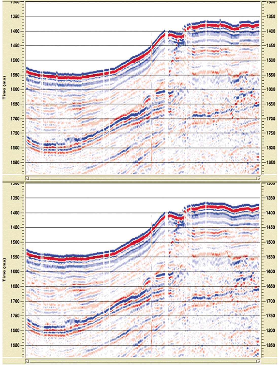
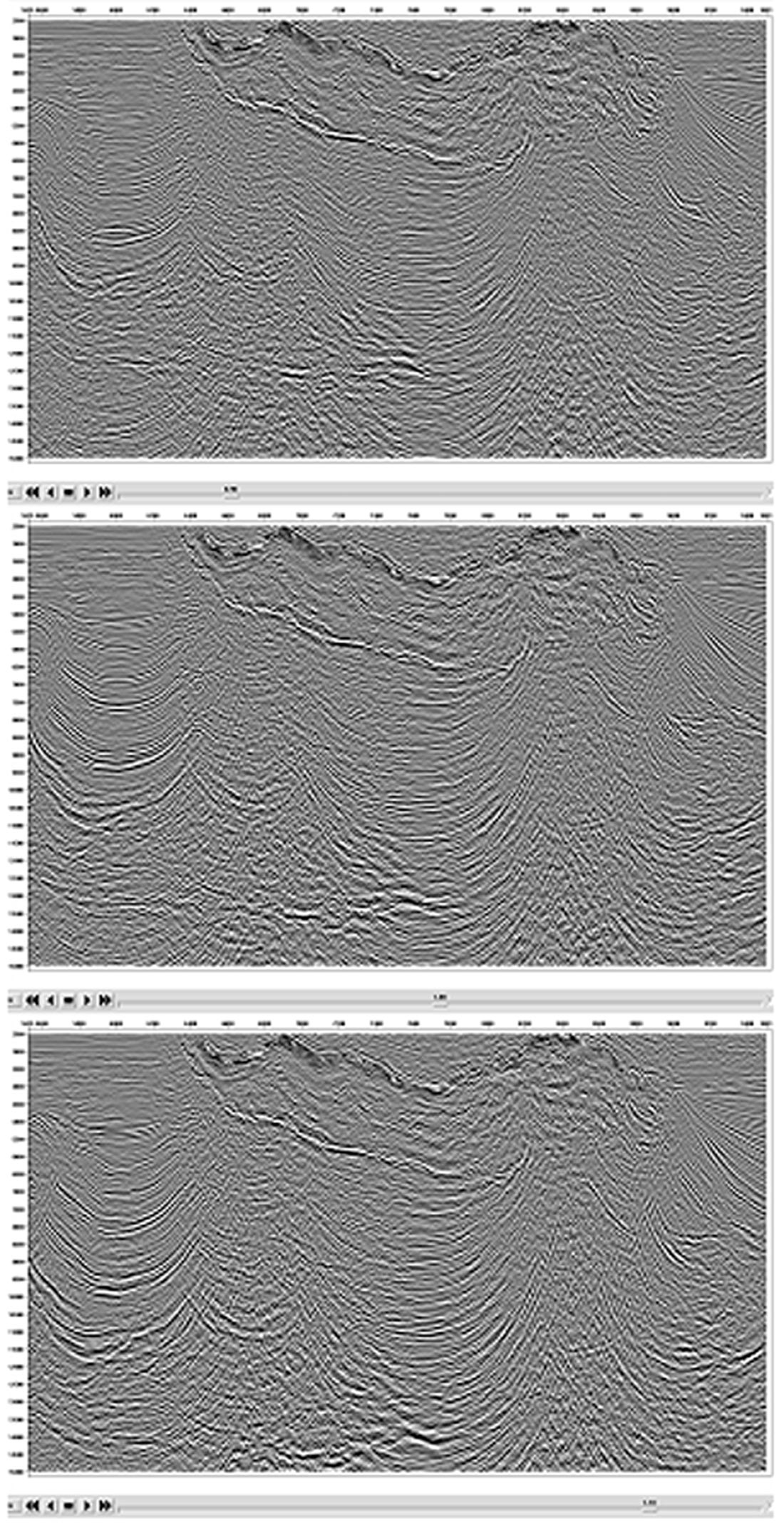
In deep water one velocity for the water layer is no longer a valid assumption. It is also likely that there will be changes in water velocity over time, for instance with underwater currents that change direction or even depth. This problem is most severe with 3D data where adjacent lines are acquired at substantially different times. The result is a substantial jitter in the cross-line direction that may contain both static and dynamic elements. This must be corrected, especially prior to any form of pre-stack migration or severe artefacts will be generated. Figure 1 shows a cross-line section from a 3D survey affected by this phenomenon on the top and after correction on the bottom.

Noise

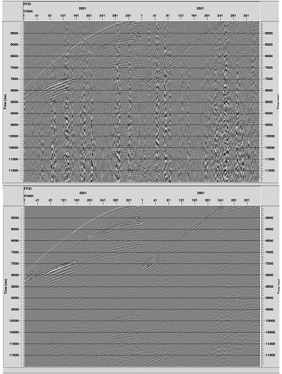
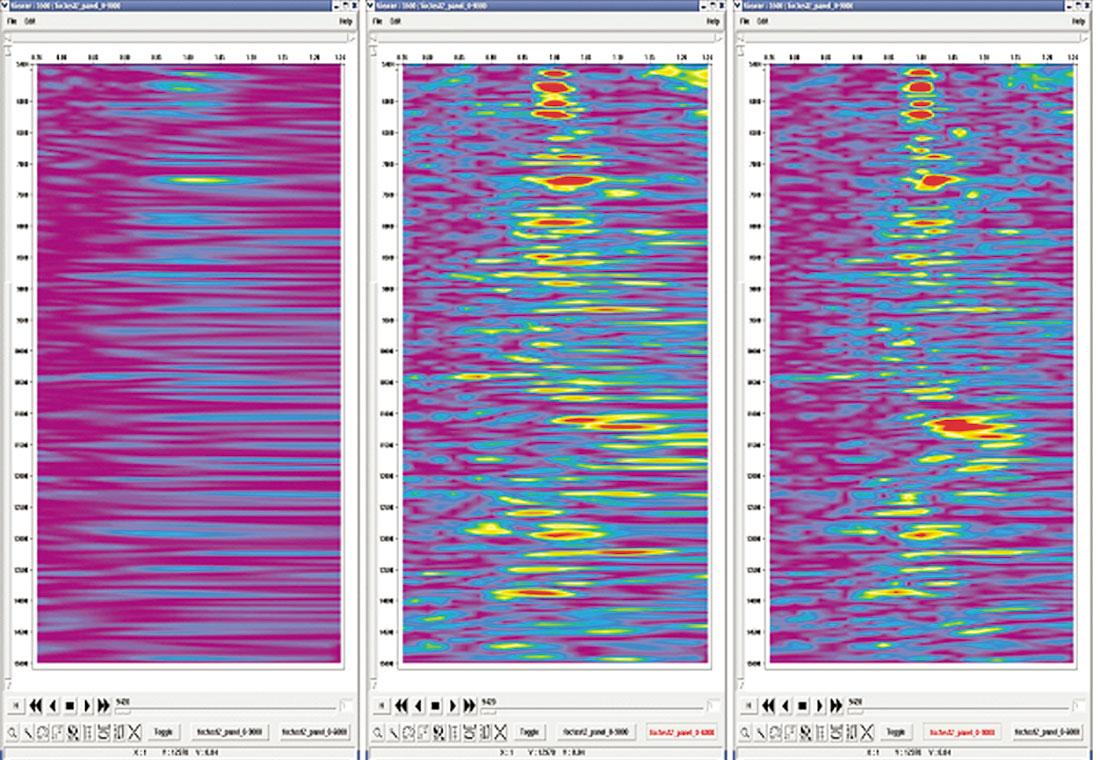
Acquiring data in deep water often implies that there is swell noise. This is due to the action of the waves on the streamer and can be quite severe in deeper water as there is less shelter from the weather and winds. An example of swell noise is shown in figure 2 (left) and after attenuation (right). Clearly this noise must be attenuated before pre-stack migration. Seismic interference must also be attenuated at an early stage, though this is common in all water depths.

Multiples

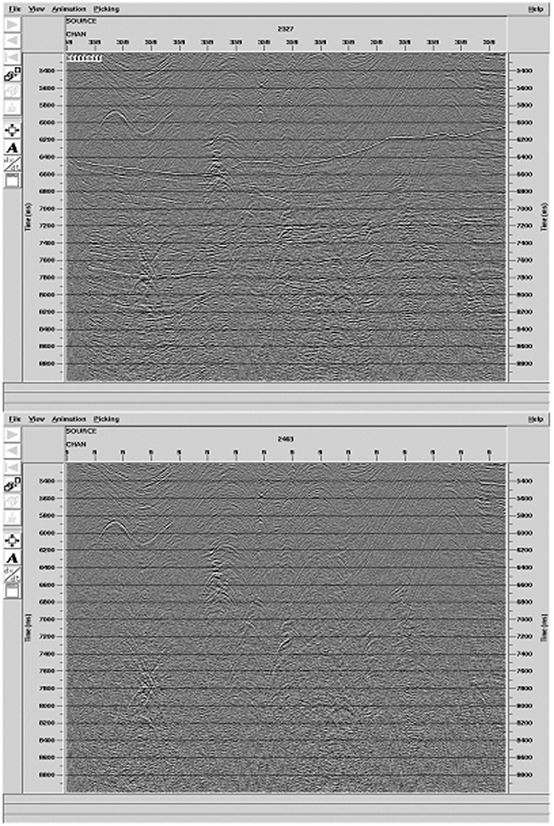
Deconvolution, an oft-used tool for multiple attenuation, is ineffective in deep water. The period of the multiple requires an operator that is approaching the length of data available resulting in statistical unreliability. Radon may be used but this requires a good estimate of the velocity. A useful combination of techniques is to first use a velocity insensitive technique such as Surface Related Multiple Elimination (SRME) developed by DELPHI. The GX Technology variant of this is termed SMA. This will remove a substantial part of the multiple reflection energy and is particularly effective on short offsets where Radon is less successful due to the smaller residual moveout. This helps to progress the data through velocity analysis and a Radon demultiple technique may be applied later using more accurate velocity information. This Radon is likely to either be a high resolution Radon or use interpolation prior to the transform. In certain areas there is diffracted multiple energy, for example in regions with rugose water velocity. In such instances an Apex Shifted Radon Transform (ASRT) can usefully attenuate this unwanted energy. Figure 3 shows an example of SMA applied to a deep-water dataset and its effectiveness on attenuating multiple reflection energy on the short offsets.

Velocity Model Building

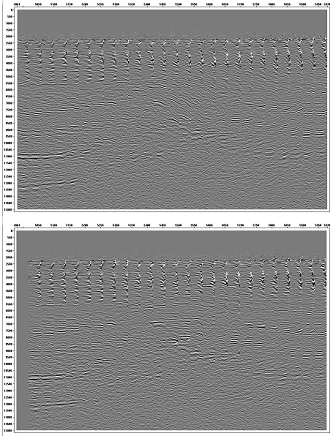
With noise and multiples attenuated it is time to start work on building the velocity model for pre-stack imaging. We will look at this process for PreSDM where the requirement is for an accurate interval velocity model. A typical process will start with some initial model. This may be a simple velocity gradient model or a model based on a velocity field used to stack the data. This will be used in an initial PreSDM to generate a set of CRP gathers. These gathers are typically subjected to an automatic event picking process, that used by GX utilizes the plane wave destructor concept to pick locally coherent events in spatial and offset coordinates. This also qualifies the data with coherency measures. This data is then fed into a tomographic inversion scheme to generate an updated interval velocity depth model. Figure 4 shows an example of RMO correction after the application of this auto-picker. Note that the gathers become flat from being substantially a long way from being flat on input. A major advantage of this approach is that it is automatic and picks every single gather. This obviously requires some computation time but it is far quicker and less biased than possible by human means. The resultant velocity field is gridded with a value at every sample in the survey. In the case of marine the water layer velocity function is assigned first and not allowed to change.

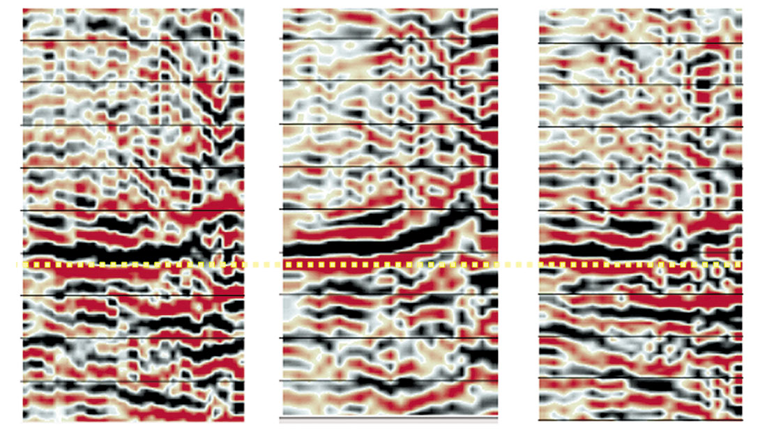
This technique works well in regions of good signal to noise and provided the offsets in the data are comparable to or larger than the depth of investigation. When the data is deeper or the signal quality poor it is necessary to use alternative methods. One such method is show in Figure 5. This shows three PreSDM sections each migrated with a percentage variation about the input velocity field. In practice it is common to use more like 11 or 15 such sections. These can be generated in 2D or 3D. The practice is to interpret these and pick a spatially variant velocity function that is then gridded for another application of PreSDM.

In practice there will be more than one pass for each of these processes. In salt provinces it is common to use the tomographic update procedure above top salt, pick the top salt, flood the salt with its velocity, migrate again, pick the base salt and proceed below the salt. Often the most useful method for sub-salt velocity analysis is to use the migration scans as gather analysis is generally problematic. The scan method may also be used with Wavefield extrapolation or Wave Equation Migration, which is particularly applicable sub-salt.

Migration Algorithms

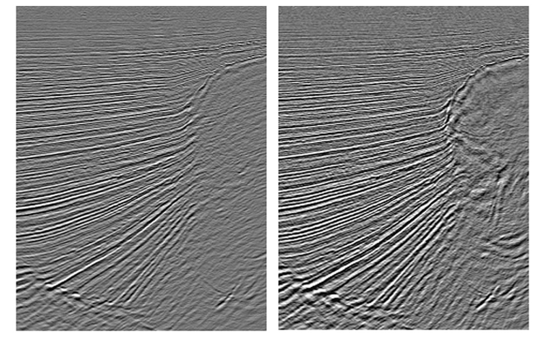
Obtaining an accurate interval velocity field is the most important element in obtaining a good result from PreSDM and it is useful to have several different tools as no one tool will work in all situations. There are also areas with specific migration algorithms may be preferred. Still the most common algorithm is the Kirchhoff method. A good implementation of Kirchhoff is capable of maintaining true amplitudes and accurately imaging steep dips. The larger the angles through which rays are allowed to bend the noisier the resultant section becomes but there are instances where very large angles are useful. One such application is to allow the rays to turn beyond 90 degrees in order to image overhanging salt domes. Figure 6 shows an example of this. The left image is obtained using a large angle but less than 90 degrees; the right image is obtained using turning rays. Clearly the turning ray Kirchhoff migration has produced a considerably improved image of the overhanging salt flank. This is not only useful from the imaging viewpoint but also from the velocity model-building viewpoint in enabling the identification of the base salt boundary.

There are instances where Kirchhoff, at least in its single arrival mode, is unable to provide as good an image as Wave Equation (or Wavefield Extrapolation) Migration. This method is generally abbreviated to WEM. WEM handles all arrivals and also handles phase better to provide less dispersion below boundaries of sharp velocity contrasts.

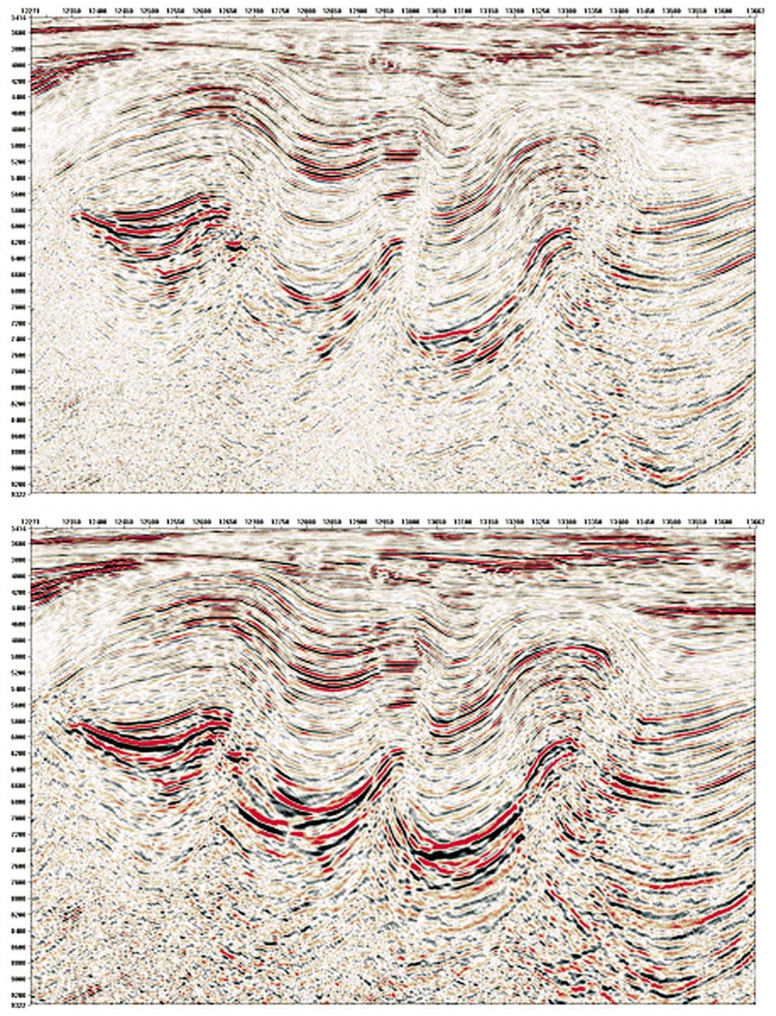
Figure 7 (see page 40) shows an example from GX Technology’s recent GulfSpan regional 2D program. In this case the WEM image has also been illumination compensated, a procedure that can be performed very accurately with this technique. It is generally not necessary to use WEM in simpler regimes but it does offer improved images beneath salt. Due to the ability of WEM to handle all paths to a particular event it will also provide improved illumination over the Kirchhoff algorithm; that is there blind spots where no data can be imaged will be smaller.

This latter point is of interest to survey design. If WEM is being considered for PreSDM after the data has been acquired then it should also be used in any illumination study that may be used to optimize the acquisition parameters.

Longer offsets and anisotropy

The importance of long offsets has been discussed. In deep water with considerable structure at deep targets this becomes very important. The presence of long offsets allows more deterministic tools such as depth domain reflection tomography to be used deeper into the section. Not only does this allow better velocity model building it also enables better application of the interval velocity as a tool in its own right. One such growing application is in using this high-resolution velocity as input to pore pressure prediction. This provides the drillers with some advance warning of where in the section they may encounter such a hazard. This is also a common issue with drilling wells in deeper water.

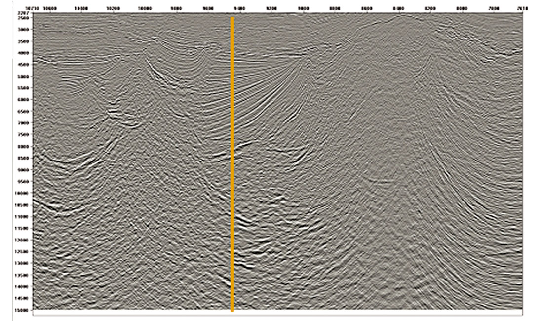
Figure 8 shows a section, again from GulfSpan with a vertical line marking a relatively complex region for velocity analysis. Figure 9 shows the CRP focussing analysis panels from this location with varying offsets. The 3km offset example is where streamers where not that many years ago, 6km offset streamers have been common until quite recently. It is clear that 6km offset gives much improved velocity resolution over 3km offset but adding yet another 3km to make a 9km streamer gives even velocity resolution.

Longer streamers have another impact. This is both awkward and useful. The longer offset data requires the use of moveout corrections beyond the simple 2-term NMO equation of long standing, to add a 4th order term. It is also possible that there will be some anisotropic behaviour in the earth requiring this formulation to be modified to include another parameter to handle this.

Anisotropy is becoming recognized as being not at all uncommon. Substantial shale beds will frequently exhibit anisotropy, as may cyclic clastic bedding. Having the longer offsets then not only forces us to deal with this issue but also allows us to more properly parameterize it. In time just one parameter (eta) is required. In depth, two parameters are required (epsilon & delta). Use of anisotropy in PreSDM allows for more accurate depth predictions. Figure 10 shows the result of applying anisotropy in PreSDM to CRP gathers. These are displayed back in time to demonstrate the gather flatness. The isotropic gather looks almost flat but in fact oscillates around being flat and results in a substantial depth error. The elliptic gathers, in this case, are at the correct depth but not flat. The anelliptic gathers are at the correct depth and flat and thus provide the best image at the correct depth. In general anisotropy in the real earth does not seem to appear in elliptic form. This is where Thomsen’s delta parameter would be equal to his epsilon parameter. The issue of azimuthal anisotropy is not addressed in this article, as this is not so specific to deep-water basins. Anisotropy in this VTI (or TTI) sense is common in many deep-water basins, generally for some part of the shallower sub-sea section. As it exists it makes sense to acquire data that enables its analysis.

Conclusions

This paper has presented some of the problems associated with imaging seismic data from deep-water basins. This is a matter of addressing several problems in a sequential fashion to get from seismic field tapes to a final image in depth. It is necessary to condition the data for velocity analysis and migration and to have a kit of tools to deal with these issues. Exploration is moving into increasing water depths and new tools are being continually developed to enable the accurate sighting of very expensive wells and avoiding drilling hazards where feasible.