Seismically Driven Characterization of Unconventional Shale Plays

Introduction

Unconventional shale plays are changing the energy sector in many ways. At the macro-economic level, shale plays are becoming a geopolitical game-changer with profound consequences for communities, energy companies, local and regional economies, and our planet. At the financial level, billions of dollars are invested each year in acquiring and developing existing and new shale plays. At the industry level we observe genuine integration of disciplines between geophysicists, geologists and engineers in order to solve the challenges posed by the shale plays. Gone are the days where the buzzword “integration” meant the ability to display well logs, seismic data and some engineering information in a 3D viewer; with shale plays, synergetic integration is an urgent necessity, applied through algorithms and workflows that combine multiple data-types to create 3D property models. This synergetic integration stems from the fact that successful development of a shale play requires the knowledge of key reservoir properties that span the spectrum of disciplines. Although each shale play is unique with its set of specific reservoir properties that control the well performances, there is a common denominator in all the shale plays that could be considered the minimum requirements for a successful development. What are these key reservoir properties that could be considered the cornerstone of any shale play?

A New Strategy for an Old Reservoir

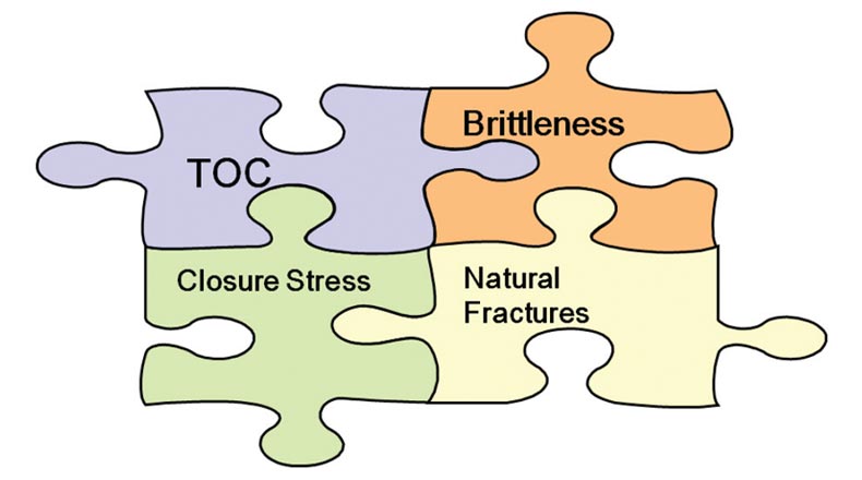
Although shale reservoirs have been producing oil and gas since the beginning of the 19th century, it is only recently that new technologies allowed for wide-spread development of these resources. Horizontal drilling combined with new fracking technologies allowed small US companies to prove the feasibility of recovering economical quantities of hydrocarbons locked in shale reservoirs, which previously were regarded as boring or as an annoying source rock. Looking back, the success of a given shale well was not solely dependent on a frack job and the industry soon discovered that a shale reservoir could be even more complex than a conventional reservoir. With most of the wells costing between 4 and 12 million dollars (mostly spent on completion), the drilling of an uneconomical shale well starts to hurt the bottom line. Efforts are underway to eliminate uneconomical wells in today’s fast-paced development programs. After a decade of rapid development within various shale plays, we are now able to identify several key reservoir properties that can have a major impact on the performance of a shale well. Although each shale play is unique, there are some general rules that are more widely applicable than others. These rules are derived from the following observations, which we might describe as the “ideal shale well”: 1) A well must be drilled in a zone that has a high TOC content thus guaranteeing the presence of oil or gas (assuming a favorable petroleum system), 2) The intercepted “shale” must be brittle enough to be fracked, 3) The induced fractures resulting from the frack job must intercept a natural fracture system and porosity, and 4) The induced fractures must remain open for a sufficient period of time to allow economic volumes of hydrocarbons to be produced. We define four key reservoir properties in an effort to simplify field development.

Key Reservoir Properties to Unlock the Shale Potential

A successful shale well usually must encounter a strata with high Total Organic Content (TOC) in order to find sufficient hydrocarbons. A “high” content means at least 4%-5%. For example in the Marcellus, Zagorski et al. (2010) showed a strong correlation between TOC and incremental increases in Gas In Place (GIP) and productivity. In many shale plays, TOC may also correlate with other rock properties such as porosity or mineralogy. In other words, knowing the TOC content and its 3D distribution in the reservoir can help estimate the distribution of one or more additional reservoir properties. This relationship between TOC and other rock properties may also work in reverse allowing for prediction of TOC through a proxy. For example, Zagorski et al. (2011) show that in the Marcellus, TOC can be inferred from gamma ray and density logs. Since gamma ray logs are readily available in all the wells, a TOC estimate is readily available. For other shale plays, a spectral gamma ray log rather than just total count gamma ray could help estimate the TOC.

Having associated hydrocarbons with regions of high TOC, the pervasive low permeabilities must now be addressed (except where natural fractures are present), which likely means hydrofracturing. The key reservoir property controlling the success of the frack job is the brittleness of the shale. In spite of the volume of fluids injected, proppant type used, and differential stress, if the shale is too ductile, we may be unable to propagate a fracture. In other words, if the shale is ductile (imagine Play-Doh© type of shale), it will not frack. There is no doubt that differential stress will play a role in determining the size and spatial distribution of the induced fractures but that can only happen in a rock that is brittle enough to propagate a fracture. The definition of brittleness varies from author to author and may take on a different meaning depending on the geography of the field and discipline of the scientist. Altindag (2003) discussed various definitions of brittleness. For the shale plays, Rickman et al. (2008) used in the Barnett shale the following definition that combines the Young Modulus (E) and the Poisson’s ratio (σ). The brittleness is assumed to have two components: one related to failure, BRT_σ , and another one related to the ability of the rock to maintain a fracture open, BRT_E.

BRT_E = (E – 1)/(8 – 1)*100
BRT_σ = (σ – 0.4)/(0.15 – 0.4)*10

The brittleness is defined simply as:

BRT = (BRT_E + BRT_σ ) /2

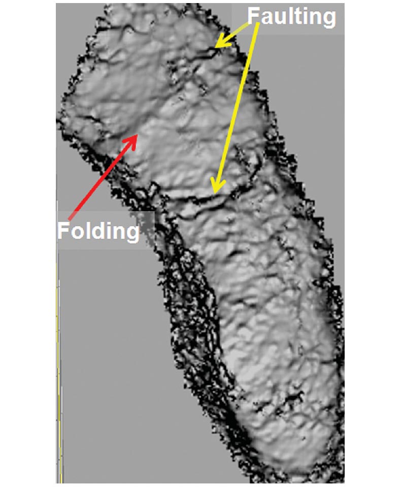
The impact of brittleness on frack jobs can be seen today when interpreting faults in many of the shale plays. Numerous outcrops show the shale mostly folding instead of faulting under tectonics forces. In the subsurface, seismic data and the use of volumetric curvature allows the identification of zones that are folded instead of being faulted (Figure 1). When estimating the porosity and mineralogy of these folded zones, we tend to discover ductile shale.

In relation to brittleness, Maxwell (2011) indicated that a recent study of more than 100 shale gas wells showed that almost half of the perforations had no production. We suspect a lack of brittleness to be the major culprit behind this lack of production, which is most likely due to a lack of induced fractures.

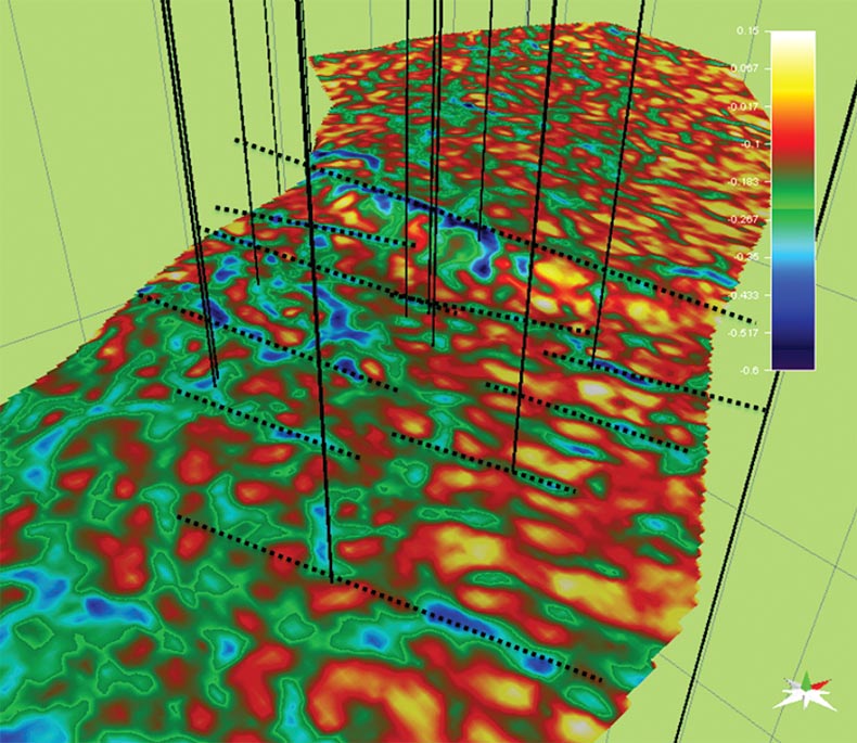
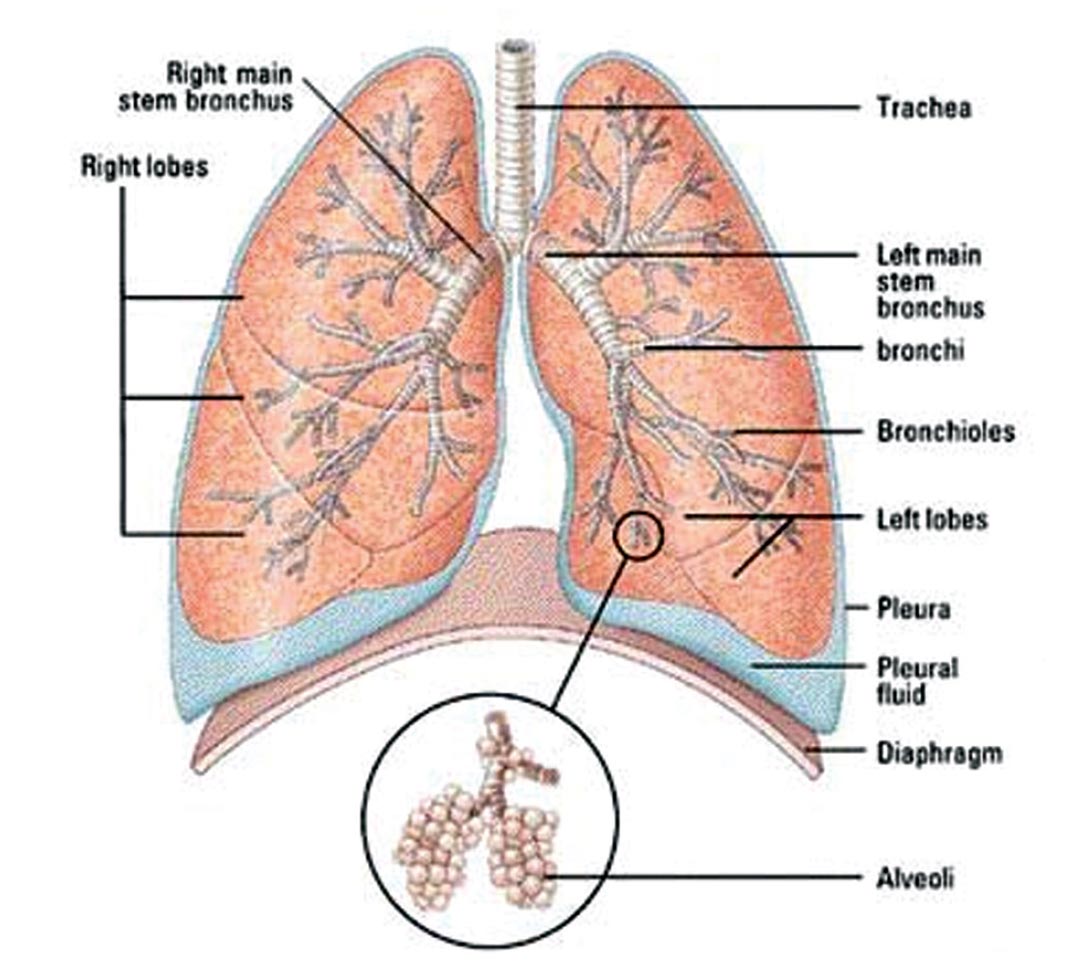
The third major reservoir property of interest is the spatial distribution of the natural fractures. Many shale reservoirs have been producing from vertical, nonhydrofractured wells for decades. For example wells 27-ShX-14 and well 203-Sh-3 at Teapot Dome, Wyoming produced more than 100,000 bbls from the Niobrara shale (Figure 2). Well 55-STX-23, located in the southern part of the Teapot Dome field, produced more than 200,000 bbls from the Steele, a genetically-similar shale above the Niobrara. Such large volumes may be explained by an extensive network of natural fractures exposing the vertical wellbore to a large, interconnected reservoir volume. The ideal frack job is the one creating induced fractures in a reservoir volume where natural fractures abound. A good analogy is the human lung (Figure 3) where the wellbore (Trachea) is connected to a large fracture (Bronchus) which is then branching into smaller fractures (Bronchi and Bronchioles) that ultimately reach the micro-fractures (Alveoli). The brittleness of the rock and the differential stress surrounding the wellbore determines mostly the dimensions of the large induced fracture (Bronchus) initiated at the wellbore. Without a connection to the natural fractures (Bronchi, Bronchioles and Alveoli), the well cannot drain a sufficient reservoir volume (causing asphyxia). This large fractured reservoir volume could hold large reserves if it has sufficient porosity. Unfortunately, a higher porosity tends to cause less fracturing.

With a network of natural fractures connecting the wellbore to a large reservoir volume and providing the necessary permeability to flow oil or gas, the last reservoir property needed to complete our ideal well is the closure stress. The closure stress (Warpinski and Smith, 1989) is given below:

Equation 1.

Where λ is the incompressibility of the rock related to fracture dilation, and μ is its rigidity related to shearing failure. σ_xx is the horizontal (closure) stress, σ_zz is the overburden stress, e_xx, e_yy, e_zz are respectively the strains in x, y and z directions. P_p is the pore pressure; B_v and B_H are respectively vertical and horizontal poro–elastic constants.

The closure stress is important since our ideal shale well that encounters a high TOC zone, that also happens to have brittle rock able to be fracked, whose induced fractures hopefully connect to an extensive natural fracture system, must remain open for an economic production to be realized. These fractures will keep their permeability if the closure stress remains low as we withdraw the hydrocarbons. If the closure stress is high, the induced fractures and the natural fracture system will close quickly.

The importance of the closure stress also implicitly points to the im portance of pore pressure which plays a major role in many shale reservoirs. The proper estimation of pore pressure is needed at all the stages of shale development and is not limited to the drilling phase. Huffman and Meyer (2011) describes a robust seismically driven pore pressure prediction workflow that provides the necessary information required for drillers, completion engineers, geo-modelers and reservoir engineers.

Depending on the shale reservoir, there may be other key reservoir properties that could play a role in field development, for example, avoiding faults in the Barnett shale. In the Marcellus, the porosity and pore-pressure are important properties required for an optimal development of the shale reservoir. In summary, the four key reservoir properties presented complete what we term the shale puzzle (Figure 4). The functional question is how to estimate directly or indirectly these rock properties in our shale reservoirs?

Useful Post-Stack Seismic Attributes for Shale Plays

Efficient development of most shale plays is bolstered through the use of seismic data. Until recently shale plays were developed with the “statistical drilling” approach: put a horizontal well in every X number of feet and “drill baby drill”. It took the operators little time to realize that well performances varied dramatically based on the statistical approach. As operators gained experienced and learned from these early intensive drilling campaigns, it become apparent that several key reservoir properties play a significant role in making economic shale wells. Symbiosis between disciplines also revealed that the key reservoir properties may be estimated from seismic data.

Notable among the post-stack seismic attributes are those derived from spectral imaging and decomposition (Castagna and Sun, 2006) and volumetric curvature (Chopra and Marfurt, 2007). Since these techniques are widely used in all shale plays, we will limit this discussion to highlight some new developments related to the volumetric curvature technology.

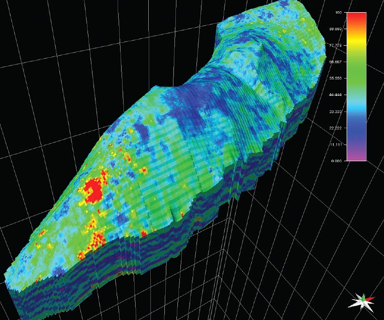
Given the importance of specific azimuths related to either major fracture orientations or the maximum horizontal stress direction, the introduction of Euler curvature (Chopra and Marfurt, 2011) allows the quantification of key orientations. Figure 5a shows the most positive curvature computed in the Niobrara interval and draped over the Niobrara horizon in the Teapot Dome. Various fault orientations are apparent but mixed together. In Figure 2, we see in the most negative curvature a possible relation between the recovered oil and faults and lineaments trending in the E-W direction. With the Euler curvature computed at zero degrees (Figure 5b), the E-W trends are clearly highlighted and allow a faster recognition of a possible relationship between the cumulative oil produced and the E-W trends. Figure 5c shows the N-S trends in the Niobrara and highlights the importance of these features in some areas of the Teapot Dome. These new directional post-stack attributes enhance the predictability of 3D fracture models derived from narrow-azimuth post-stack seismic attributes.

Spatial resolution of volumetric estimates of curvature may be increased through the use of spectral inversion. Since shale plays require a detailed description of the faults, the relative impedance resulting from the spectral inversion provides a high level of detail unseen on the original seismic. Chopra et al. (2006) includes examples of highly-detailed stratigraphic descriptions derived from spectral inversion. When spectral inversion is coupled with volumetric curvature the imaging of small faults is improved, as shown on the Barnett shale example (Figure 6) where faults play a major role in the well performance.

These attributes do not provide a direct estimate of any of the four attributes described in the previous section but they will be used in the continuous fracture modeling approach to estimate the spatial distribution of fractures. These post stack attributes could be further enriched with others derived from pre-stack seismic. A powerful approach that optimizes the use of pre-stack data is described in the next section.

Pre-Stack Seismic and Extended Elastic Inversion (EEI): A Powerful Tool for Solving the Shale Puzzle

The use of pre-stack data in reservoir characterization is not new but has mostly been limited to facies and fluid discrimination. With shale plays and the pressing need to derive elastic properties, pre-stack seismic data are becoming the cornerstone of the shale solution and the key to deriving the four rock properties described earlier. Turning the pre-stack seismic data into elastic properties that can be used by geologists and engineers requires an inversion technique. The Extended Elastic Inversion (EEI) is a powerful tool that provides key features not found in other prestack inversion techniques.

Whitcombe et al. (2002) proposed the EEI technique that has many critical benefits for the shale plays. Since the EEI technique inverts separately the near, mid and far offsets, any inversion technique may be used to invert the angle stacks. The need for high resolution seismic attributes in shale plays is critical thus we propose the use of stochastic (or geostatistical inversion) on each stack. Stochastic inversion yield estimates of Vp, Vs, and density with a sampling on the order of log data, which in turn will lead to high resolution elastic properties.

Another major benefit of EEI coupled with geostatistical inversion is the ability to quantify uncertainties based on standard deviation of multiple equi-probable outputs. These realizations are used to compute average elastic properties but also will lead to a quantitative evaluation of their uncertainties through the use of probability functions.

The EEI is defined as:

where

Equation 2.

Where α is the P-wave velocity, β is the S-wave velocity, and ρ the Density. The exponents p, q, and r are defined as follows:

Equation 3.

Equation 4.

Equation 5.

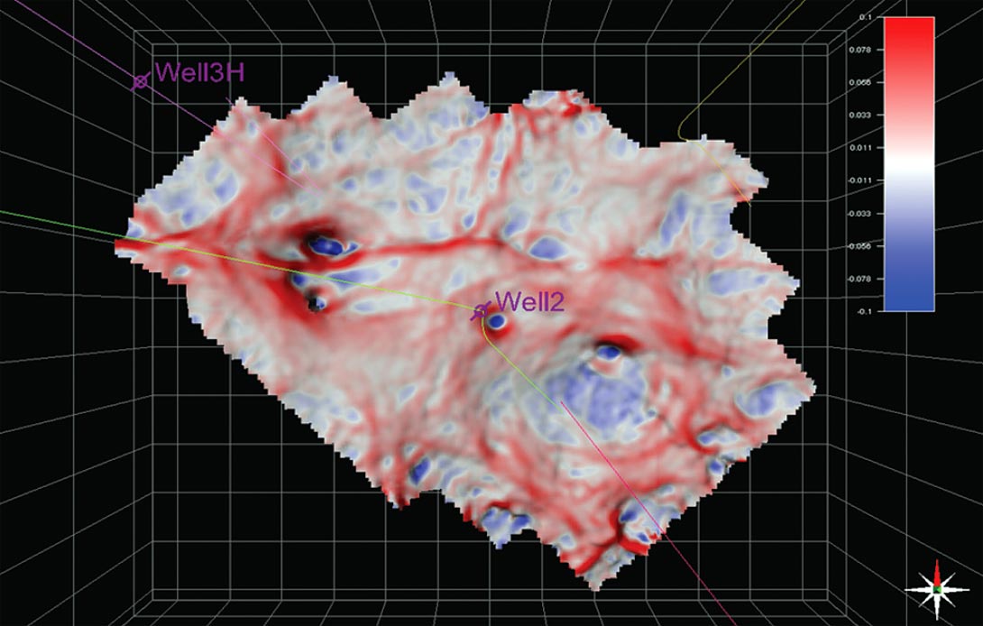
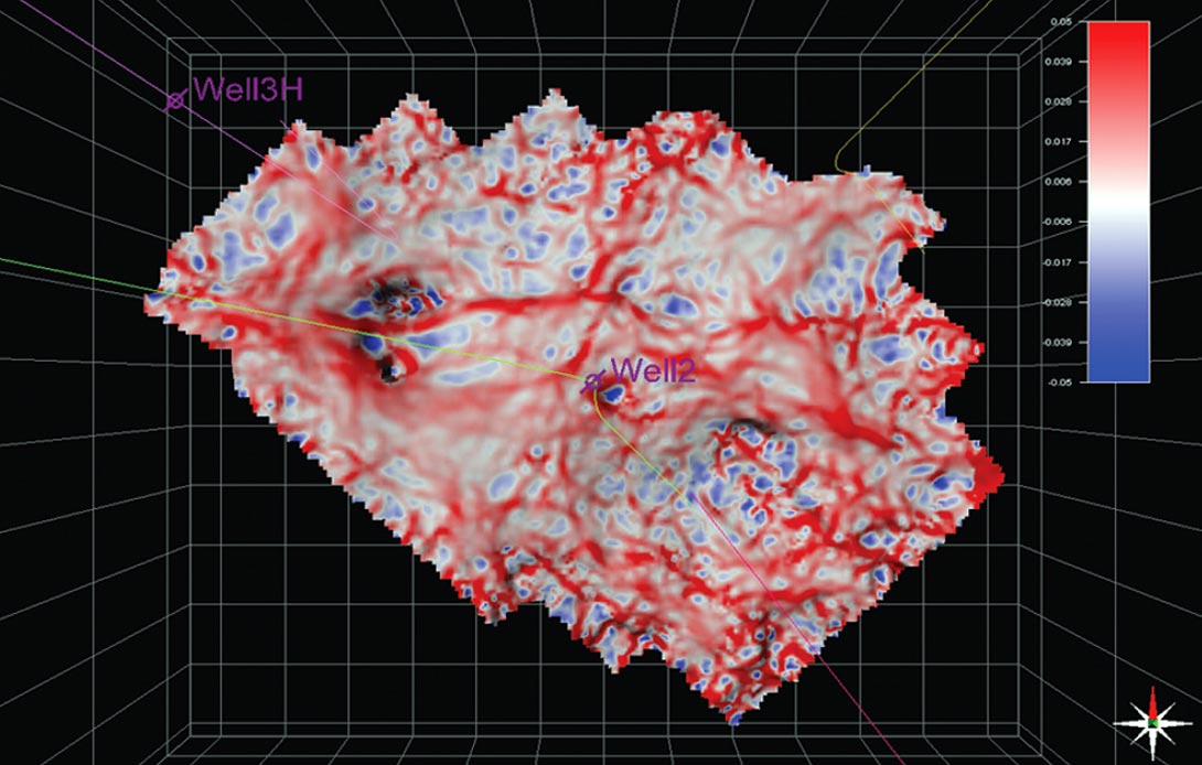
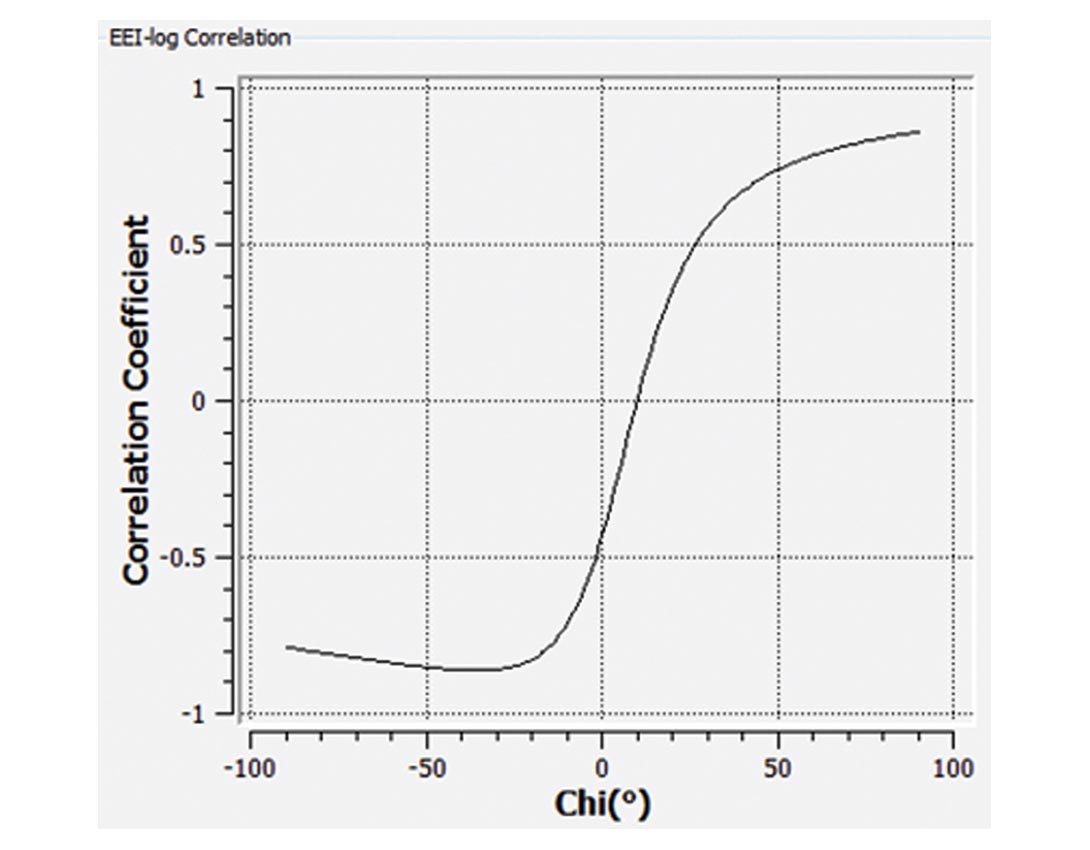
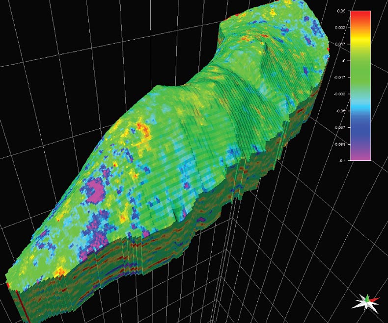
The other powerful feature of the EEI comes from the use of the χ angle. The main difference between extended elastic impedance and normalized elastic impedance (Whitcombe, 2002) is the change of variable from sin(θ) to tan(χ). This change of variable allows for calculation of impedance values beyond physicallyrealizable angles. As shown by Whitcombe et al. (2002), certain values of χ produce extended elastic impedance that correlates well with rock properties, such as lambda, mu, bulk modulus, and Vs/Vp ratio. Additionally, one may determine empirically a χ angle that correlates well with other log curves, such as gamma ray, porosity, or water saturation (Whitcombe et al., 2002). Once the compressional velocity, shear velocity, and density cubes are computed from the extended elastic impedance, other “rock property” cubes can be calculated using the appropriate value of χ. Since we noticed that key reservoir properties such as TOC could be inferred from other logs such as gamma ray in the case of the Marcellus shale, the EEI provides the unique opportunity to invert directly for gamma ray thus providing a seismic estimate of TOC. For example in the Niobrara reservoir at Teapot Dome, the porosity is correlated to the χ angle as shown in Figure 7. This correlation is the highest when χ is equal to -30 degrees. Using this value in the EEI results will lead to the direct inversion of porosity (Figure 8) at a very high resolution since all the EEI results are derived from the stochastic inversion sampled at 1 ms or less. Based on various projects using the EEI we have successfully found high correlations between the χ angle and gamma ray, porosity, resistivity, water saturation and other reservoir properties.

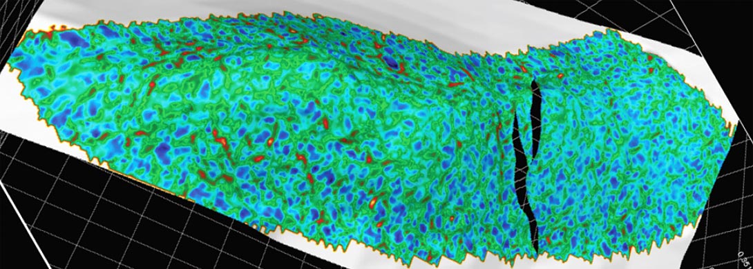
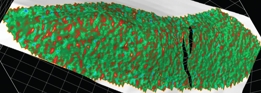
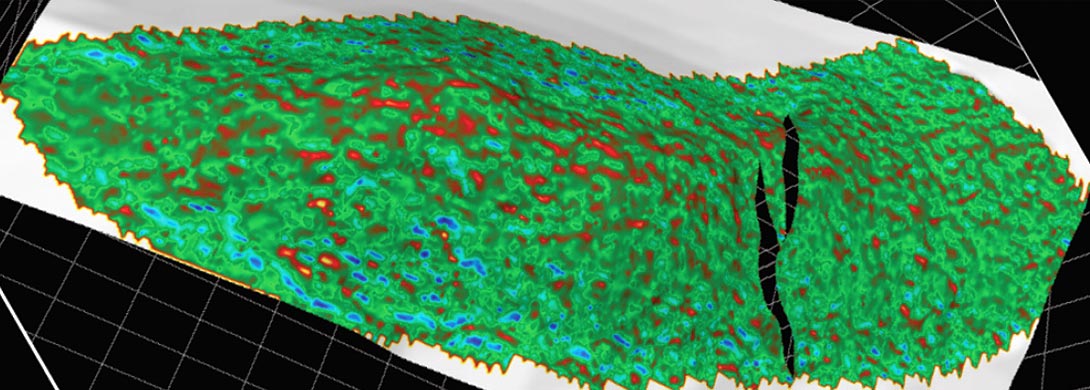
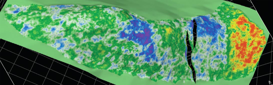
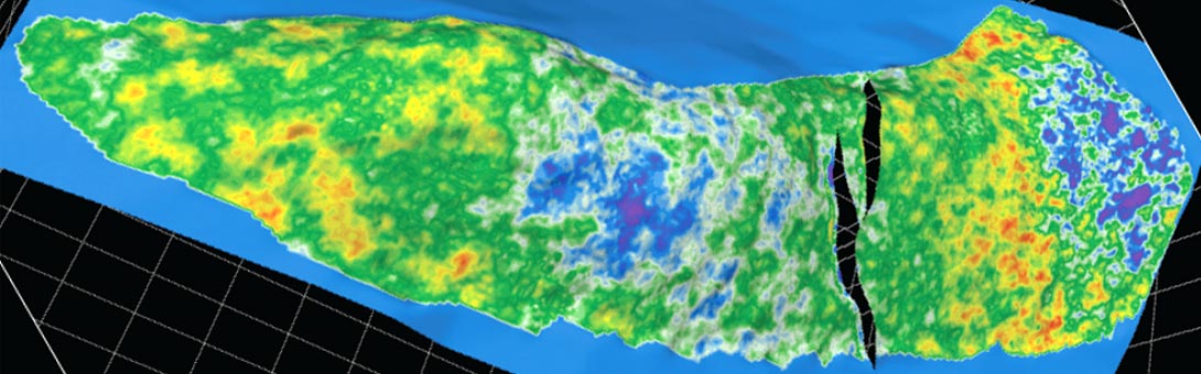
In addition to specific χ angles related to particular logs, the EEI provides Vp, Vs and density at a high resolution since the stochastic inversion was used. From these basic cubes all the elastic properties will be computed, including Young’s Modulus (E) and the Poisson’s ratio (σ), which are used to compute brittleness estimates (Figure 9). To better illustrate important variations that occur in the brittleness, average maps are computed in the Steele (Figure 10a), Upper Niobrara (Figure 10b) and Lower Niobrara (Figure 10c) at Teapot Dome. From these maps one can see significant vertical and lateral variations. These variations have important implications on the natural fracture system and effectiveness of hydrofracturing.

One observation worth mentioning is that in Wyoming the Lower Niobrara seems to be more brittle than the Upper Niobrara, which is a major target for many operators actively drilling the DJ Basin in Colorado. In other words, the shale plays vary dramatically and lessons learned in one area may not apply at all in other areas. The best strategy to overcome these variations is to use a seismically driven approach that provides a quantitative description of lateral and vertical variations, representative of local geology.

The EEI results could be used to compute incompressibility (λ), and rigidity (μ). A first approximation for the closure stress is the leading term [λ / (λ + 2 μ)] that can be estimated directly from the EEI results. A more accurate estimation of the closure stress requires the estimation of the pore pressure P_p.

Out of the four key properties required for a better understanding of the shale plays, three of them can be estimated from the EEI results. The last key property is the spatial distribution of the natural fracture system where both the EEI results and the post-stack attributes will be used simultaneously.

High Resolution Fracture Density Models Estimated from the Continuous Fracture Modeling (CFM) Approach

In order to capture fracture effects at multiple scales and simultaneously integrate the available core, log, seismic, and well test data information, the Continuous Fracture Modeling™ (CFM) approach (Ouenes et al. 1995; Ouenes, 2000; Ouenes et al., 2010) is used to produce predictive models that are validated with blind wells, actual drilling and reservoir simulation. The CFM approach does not focus on identifying the fractures themselves but rather on identifying the factors that control where fracturing occurs. It is common knowledge that brittleness, structure, proximity to faults, and other geological factors control the location and intensity of fracturing. These factors, known as fracture drivers, can be identified using seismic data (available in the inter-well space) as well as borehole data. These fracture drivers are then related to fracture indicators, demonstrating the existence of a fracture at a specific location in a well. The fracture indicators are derived from interpretation of core descriptions, image logs, production logs, et cetera. Once the relationship between fracture drivers and fracture indicators in the wells is established, the fracture drivers can be used to predict the location of fractures in the inter-well space.

A neural network is used to find possible relationships between fracture drivers and fracture indicators observed at the wellbore. The neural network approach first ranks all the fracture drivers according to how reliably they correlate with the fracture indicators. The modeler then reviews the results in light of what is known about the significance and robustness of each fracture driver, and how the ranking compares to what is understood about the physical distribution of fractures in the reservoir. The best-correlated fracture drivers that make sense geologically are then subjected to a training and validation process before being used to generate a suite of equi-probable fracture density realizations. These realizations can then be screened and calibrated to permeability-thickness (kh) data obtained from well tests if available. The resulting effective permeability model can then be exported for use in numerical simulation and development planning.

Since its inception in 1995 (Ouenes et al., 1995) the main focus of the CFM approach has been to incorporate multiple seismic attributes to improve the 3D description of fractures. The availability of new seismic attributes continuously improves the predictive capabilities of the CFM models. The addition of acoustic impedance, spectral imaging attributes, and volumetric curvatures (Jenkins et al., 2009) into the list of drivers significantly improves estimates of fracture density, even when only post-stack seismic information is available.

The use of elastic properties derived from pre-stack EEI is one of the more robust seismic inputs for the CFM approach (Bejaoui et al., 2010). Because of the flexibility and versatility of the CFM approach, it will continue to benefit from new seismic technologies that provide better descriptions of subsurface properties.

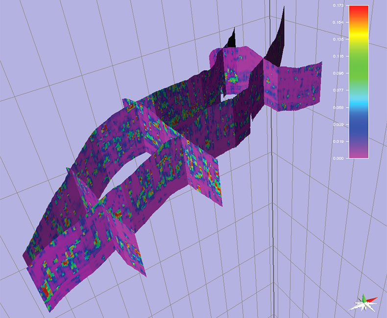
Figure 11 shows a fence diagram illustrating lateral and vertical variations of a 3D fracture density model derived by the CFM approach in the Steele and Niobrara shale at Teapot Dome. The derivation of this model required the use of image logs interpreted at three wells, 3D geologic models constrained by seismic, and multiple seismic attributes including spectral imaging attributes, volumetric curvatures including three Euler curvatures, and the results from EEI high-resolution pre-stack inversion. The ranking of attributes shows the importance of the EEI derived attributes such as brittleness, which is expected since these attributes provide a direct indication of the rock properties that may affect fracturing.

With the estimation of the 3D fracture density, the basic four pieces of the puzzle have been defined; it is now up to the development team to put them together into a drilling plan.

Putting it all Together

When the four key reservoir properties are available, geobodies may be used to satisfy one or multiple conditions. For example a landman would like to have a map showing the high TOC areas that he can lease. This map could be derived by applying a cutoff on the 3D TOC distribution and computing the net thickness of the reservoir zones that have a TOC higher than the cut-off. The exploration or asset manager would like to have more than just a TOC net thickness map and will be interested in the same map applied to both the brittleness and fracture density to upgrade or downgrade drilling areas. A 3D geobody showing the best zones where two or even three of the key properties have optimal values will highlight the zones of interest. The completion engineer would benefit from the combination of the brittleness and closure stress models to design his frack jobs. Using the 3D models of brittleness and closure stress, selective fracking is becoming possible and may dramatically reduce the cost of a shale drilling program as well as mitigate potential environmental impact by reducing the number of frack stages. With mini-earthquakes (probably resulting from frack jobs) alarming communities and realizing that less than 10% of the fluids and proppants are making it into shale reservoirs, maybe it is time to stop using brute-force along the entire wellbore and selectively frack only the best rock. The fast-paced and high-profile nature of the shale boom may benefit from seismically-driven reservoir characterization, so long as the proper pieces of the shale puzzle are put into place.

Acknowledgements

The author would like to thank Raul Cabrera and Allan Huffman for the ThinMan™ discussions and input for the Barnett shale example. The contribution of Douglas Klepacki, Chad Baillie and Amares Aoues to the CRYSTAL™ geophysical tasks in the Teapot Dome project, and the editorial comments of Kevin McKenna and David Close are greatly appreciated.