Seismic Inversion – The Best Tool for Reservoir Characterization

Introduction

The principle objective of seismic inversion is to transform seismic reflection data into a quantitative rock property, descriptive of the reservoir. In its most simple form, acoustic impedance logs are computed at each CMP. In other words, if we had drilled and logged wells at the CMP’s, what would the impedance logs have looked like? Compared to working with seismic amplitudes, inversion results show higher resolution and support more accurate interpretations. This in turn facilitates better estimations of reservoir properties such as porosity and net pay. An additional benefit is that interpretation efficiency is greatly improved, more than offsetting the time spent in the inversion process. It will also be demonstrated below that inversions make possible the formal estimation of uncertainty and risk.

In various forms, seismic inversion has been around as a viable exploration tool for about 25 years. It was in common use in 1977 when the writer joined Gulf Oil Company’s research lab in Pittsburgh. During this time, it has suffered through a severe identity crisis, having been alternately praised and vilified. Is it just coloured seismic with a 90 deg phase rotation or a unique window into the reservoir? Should we use well logs as a priori information in the inversion process or would that be telling us the answer? When should we use inversion and when should we not? And what type: blocky, model-based, sparse spike? At Jason Geosystems we offer all these algorithms - and a few more. In the following, I will briefly discuss them in a somewhat qualitative manner, keeping the equations to a minimum. After all, it is drilling results which count and against which any algorithm will ultimately be measured.

The Inversion Method

The modern era of seismic inversion started in the early 80’s when algorithms which accounted for both wavelet amplitude and phase spectra started to appear. Previously, it had been assumed that each and every sample in a seismic trace represented a unique reflection coefficient, unrelated to any other. This was the so-called recursive method. The trace integration method was a popular approximation. At the heart of any of the newer generation algorithms is some sort of mathematics - usually in the form of an objective function to be minimized. Here I will write that objective function, in words, rather than symbols and claim that it is valid for all modern inversion algorithms - blocky, model-based or whatever.

Obj = Keep it Simple + Match the Seismic + Match the Logs (1)

Let’s look at each of these terms, starting with the seismic. It says that the inversion impedances should imply synthetics which match the seismic. This is usually (but not always) done in a least squares sense. Invoking this term also implies a knowledge of the seismic wavelet. Otherwise, synthetics could not be made. At this point, life would be good except for one thing. The wavelet is band-limited and any broadband impedances that would be obtained using the seismic term only would be nonunique. Said another way, there is more than one inversion impedance solution which, when converted to reflection coefficients and convolved with the wavelet would match the seismic. In fact there are an unlimited number of such inversions. Worse, such one-term objective functions could even become unstable as the algorithm relentlessly crunches on, its sole mission in life being to match the seismic, noise and all, to the last decimal place.

Enter the simple term. Every algorithm has one. It could not care less about matching the seismic data, preferring instead to create an inversion impedance log with as few reflection coefficients as possible. Different algorithms invoke simplicity in different ways. Some do it entirely outside of the objective function by an a priori “blocky” assumption. In our most-used algorithm it is placed inside the objective function in the form of an L-1 norm on the reflection coefficients themselves. This is advantageous since it locates all the important terms together where their interactions can easily be controlled. How much simplicity is best? The answer is project-dependent and will be different for example, for hard-contrast carbonates and soft-contrast sands and shales. We exercise control by multiplying the seismic term by a constant. When the constant is high, complexity rules. When it becomes smaller, the inversion becomes more simple with a sparser set of reflection coefficients. I will now attach the name sparse spike to these types of inversions.

What about the “Match the Logs” term? When turned on, it makes the inversion somewhat model-based. Sounds reasonable - the inversion impedances should agree or a least be consistent with an impedance model constructed from the well logs. And it is reasonable, as long as it is not overdone. The primary use of the model term should be to help control those frequencies below the seismic band. When it is used to add high frequency information above the seismic band, great care should be exercised (more on this below). We control the model contribution in a variety of ways both inside and outside of the objective function. In the initial iteration of a sparse spike inversion, the model term is set firmly off. We need to very clearly isolate the unique and separate contributions of the seismic and the model. In the final inversion, we may turn it on to achieve the best power matching between the model and seismic at the transition frequency.

By now you might be thinking that no simple label can be applied to any modern algorithm. You would be right, and as we will see below, the distinctions can become even more blurred.

The Details - Low Frequencies, Constraints, QC, Annealing, Global Inversion

It is important how the low frequency part of the inversion spectrum is computed. By low, we mean the frequencies below the seismic band. They are important since they are present in the impedance logs which we seek to emulate. Commonly, the low frequencies are obtained from an impedance model derived from the geologic interpolation of well control. They can be added to the inversion afterwards as an end step or within the objective function itself. In the latter case only very low frequencies need to come from the model. At Jason, we can do both and each has its advantages. Whichever method is used, you might now be saying that all inversions must, to some degree, be model-based. The writer would not dispute this assertion. The important point though, is that the model contribution is essentially in a different band than that of the seismic.

There are other strategies in seismic inversion which control the way in which the output impedances are obtained. It is common to define high and low limits on the output impedances. These are supposed to keep the inversions physical and consistent with known analogues and theories. Our implementation is unique in that these constraints are not a fixed percentage of the log impedances but can be freely defined at each horizon, variable with time. The constraints are interpolated along the horizons throughout the project, riding them like a roller coaster. Could the inversions be then critically dependent upon inaccurate horizons interpreted from seismic data? We address this potential problem in two ways. In the first pass of inversion, the constraints are relaxed to allow for inaccuracies. The horizons are then re-evaluated against the initial inversion before a final pass with tighter constraints. Second, the re-evaluation can be done on an inversion without the model-based low frequencies added in at all. We call this the relative inversion and it is by definition, free from any inaccuracies in the input model.

Quality control of the relative inversion comes from perhaps an improbable source. In our sparse spike approach, when we invert at the well locations, the impedance log is not made available to the algorithm. Only the user constraints and the objective function settings control the output, leaving it free to disagree with the logs. It then follows that comparing the relative inversion and the band-limited impedance logs is a very powerful quality control tool. The corollary is that the addition of more logs to the inversion project increases confidence in the result rather than copying the answer into it.

Some algorithms incorporate a process called simulated annealing. This method deliberately takes a round-about path to the solution of the objective function in recognition of the fact the solution space may not contain a single simple minimum - the inversion solution. If the solution space is a bumpy place, then simulated annealing is indeed needed to avoid being hung up on local minima. So, is solution space bumpy or not? It depends upon how the inversion problem is parameterized. In the Jason sparse spike algorithm family, the parameterization is by impedance and grid point, resulting in a solution space without local minima. Some algorithms parameterize by impedance and time. That is a more problematic parameterization due to the fact that the time parameter can be strongly non-linear,. The result is a much more complicated solution space which may necessitate the use of a simulated annealing algorithm to come to a meaningful solution.

Global is another term which has recently been used in conjunction with inversion. In Global mode, more than one trace is inverted at the same time within a common objective function. The idea is that seismic noise induced variations that are not consistent over a user-specified number of traces will tend to be suppressed in the output impedances. The result is a smoother looking inversion, which, if one has been careful, does not compromise resolution. The number of traces inverted at once varies with algorithms. We typically simultaneously invert for large, slightly overlapping blocks of traces, the only limit being imposed by CPU memory.

In the preceding, our discussion has been centred on inversion methods which emphasize sparsity as a way to invoke the ‘keep it simple’ term. In the following, we present some field examples of this and other inversion methods, some with potentially even more powerful strategies.

Examples

Constrained Sparse Spike Inversion

This is the most common inversion algorithm in use by our clients. Most importantly, they need to understand precisely what statement the seismic data, itself is making about impedance. Sparse Spike is ideally suited for this since, among its other virtues (noted above), it produces both a relative (no low frequencies information from the logs added) and an absolute (low frequencies added) version. The separate contributions of the logs and the seismic are then clear.

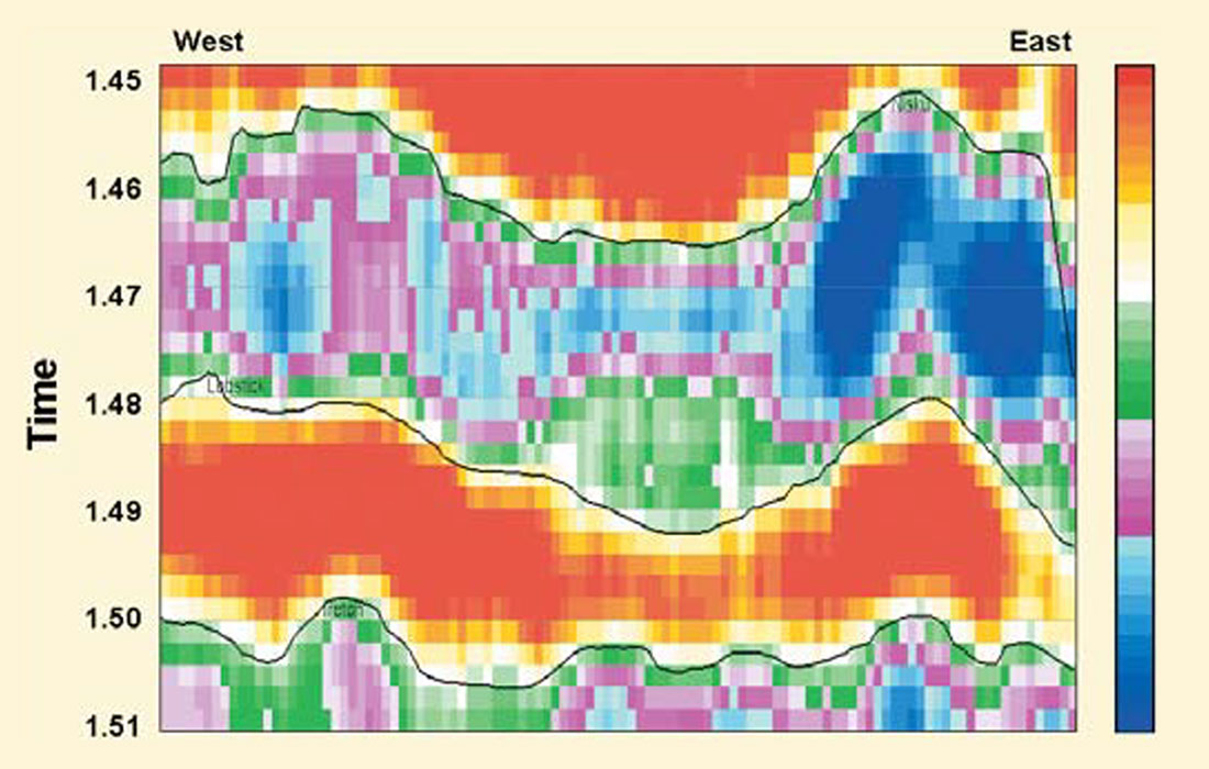
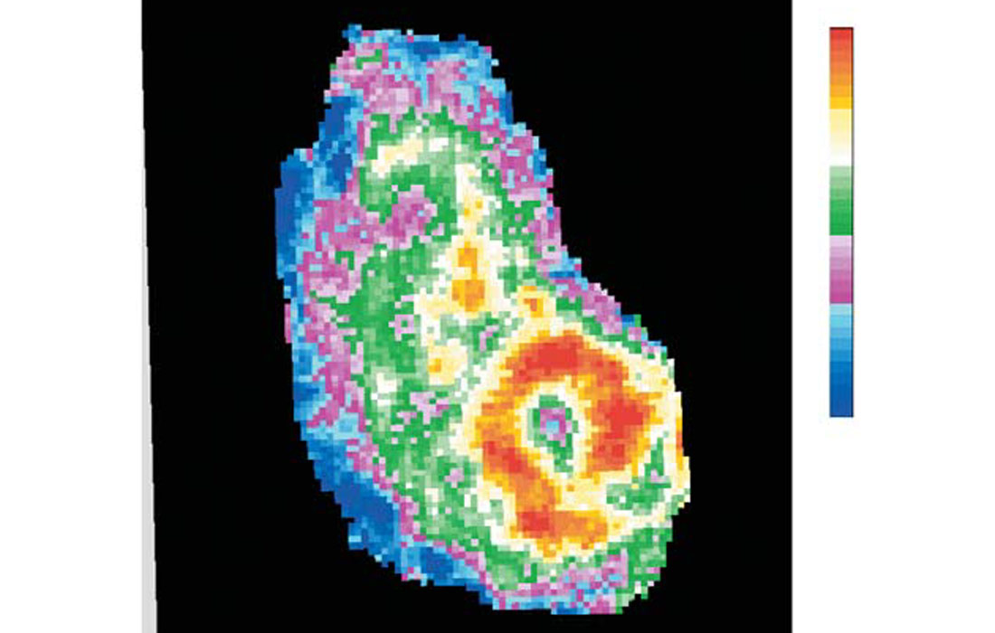
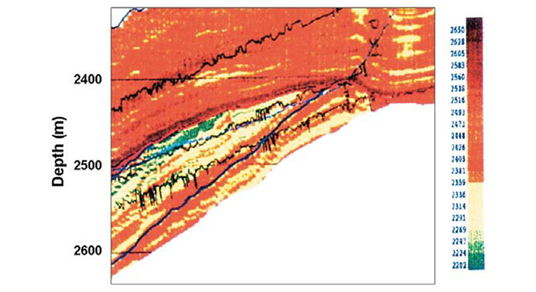
Figure 1 shows such an inversion over a Nisku reef. On structure, the blue colours represent the low impedances of the porous reef which has both a west and an east build-up. Farther to the east are low impedance shales. The plot is in an un-smoothed format so that the contribution of each voxel (small rectangle) can be more easily seen. Meaningful lateral variations in impedance of 1 or 2 samples have been achieved and variations in impedance within the reef can be identified. The inversion volume was converted to depth using a client-provided depth datum, its associated time datum from the inversion and velocities from the geologic model. The depth inversion was then converted to porosity using the observed relation in the logs. Maps of average porosity were made for several depth intervals and one of these is shown in Figure 2. The best porosity is concentrated in the south-east reef but in a non-homogeneous way. Wells were drilled from these maps and confirmed the inversion predictions.

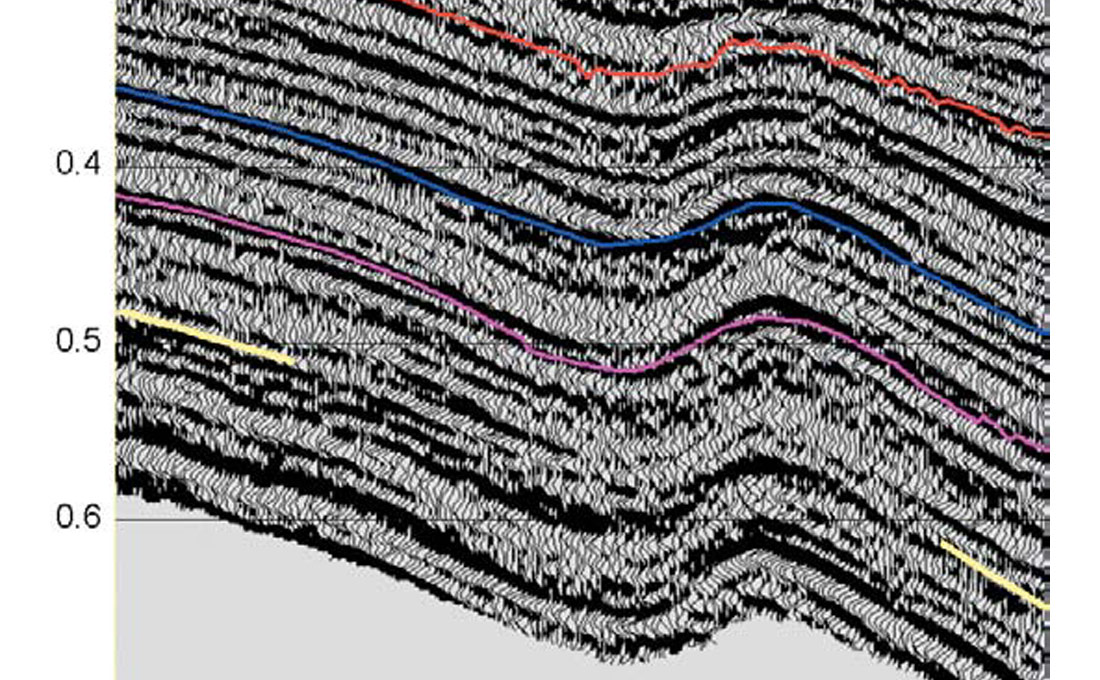
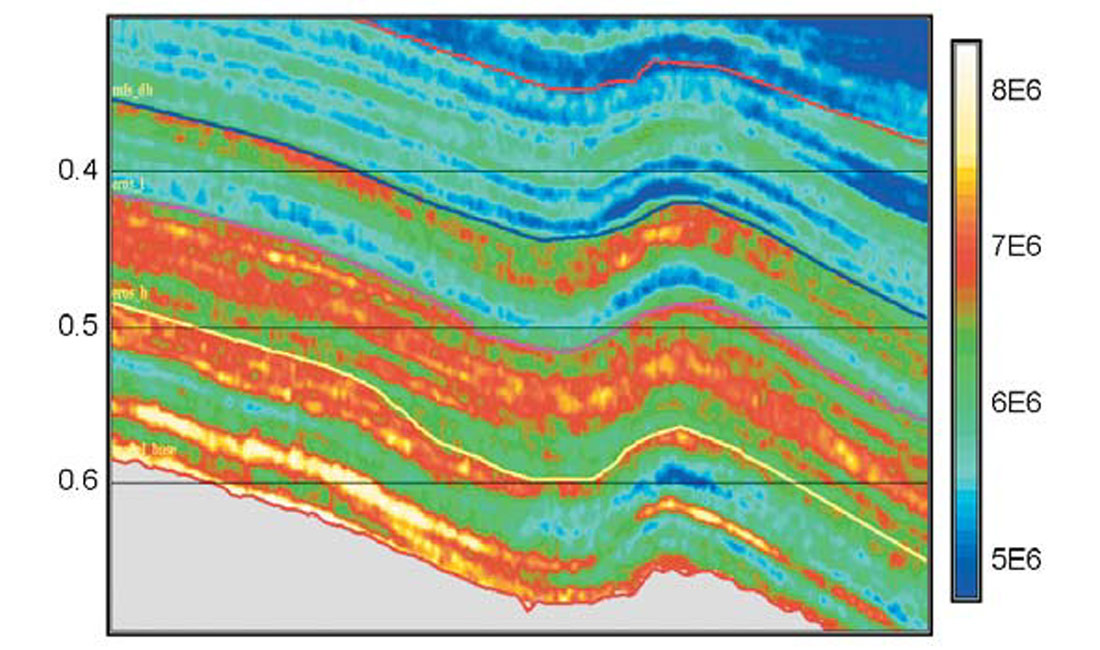
In Figure 3 we show a southeast Asia clastic example from Latimer et al., 1999. The facies are an alternating sequence of sands and shales. Interpretation is problematic due to the close vertical positioning of contrasting layers within half of a wavelet length. The result is severe interference (tuning) and a general complication of the seismic section. The interpretation of the yellow reservoir event is particularly difficult. Figure 4 shows the inversion result. It is generally more simple and the interpretation of the yellow event is obvious. It is now interpreted as a sequence boundary which is overlain by an incised valley sand.

Model-Based Inversion

We reserve the term ‘model-based inversion’ for methods that attempt to achieve resolution within and beyond the seismic band by a stronger use of the a priori impedance logs in the model term of equation 1. In one of the model-driven methods we support, the simplicity term is implemented by limiting the solution space to that spanned by (perturbed) well logs. The model term is free to act both within the seismic band and outside of it. Obviously we need to have confidence in our logs and in the relation between them and the seismic data if we are going to use them in such a way. This confidence is generally provided by running a sparse spike inversion first. As in any model-based approach we need to ensure that all possible facies are represented in the logs. The Jason inversion works by adapting the initial model made from a simple interpolation of the input logs along structure to a more detailed one. At any given CMP to be inverted, an optimal weighting of the input wells is determined to minimize the residual between the input seismic and the inversion synthetic. The whole operation is performed in a transformed principle components space to remove non-uniqueness resulting from the similarity of input wells. The final detailed model is also the output inversion. Since high resolution logs are input, high resolution in the inversion is possible.

This approach has been used successfully by Helland-Hansen et al., 1997 in the North Sea to highlight regions where sands might occur with increased probability. Figure 5 shows the input density model constructed from selected wells in principle components space. Figure 6 shows an enlarged section of the final model where the green colours represent densities indicative of increased sand probability. Prior to doing the inversion, this area had not been considered to be sand prone. A well was drilled on this anomaly and the inferences from the inversion were confirmed. This resulted in the development of a new productive horizon. The model-based algorithm has two flavours. The second, not illustrated here, associates character changes in (multiple) seismic data set(s) with well log attributes and obviates the need for a wavelet.

Geostatistical (Stochastic) Inversion

Geostatistical simulation differs from all of the other methods in one respect. There is no objective function and hence no need for a simplicity term to stabilize it. Rather, property solutions (impedance, porosity, etc.) are drawn from a probability density function (pdf) of possible outcomes. The pdf is defined at each grid point in space and time. A priori information comes from well logs and spatial statistical property and lithology distributions. As in the other model-based methods, the logs are assumed to represent the correct solution at the well locations. It is again useful to run a sparse spike inversion first, to establish this. Historically, away from wells, geostatistics has had problems. It is the inversion aspect of geostatistics which has finally guaranteed its use as a modern inversion tool. The geostatistical (or stochastic) inversion algorithm simply accepts or discards simulations at individual grid points depending upon whether they imply synthetics which agree with the input seismic. The decision to accept or reject simulations can optionally be controlled by a simulated annealing strategy. The inversion option results in a tighter set of simulations, the variation of which can be used to estimate risk or make probability maps. The simulations can be done at arbitrary sample intervals. Close to wells, resolution beyond the seismic band can reasonably be inferred. Away from wells, the absence of a simplicity term in the simulation and the statistical conditioning still hold the possibility of resolution beyond that of traditional inversion methods.

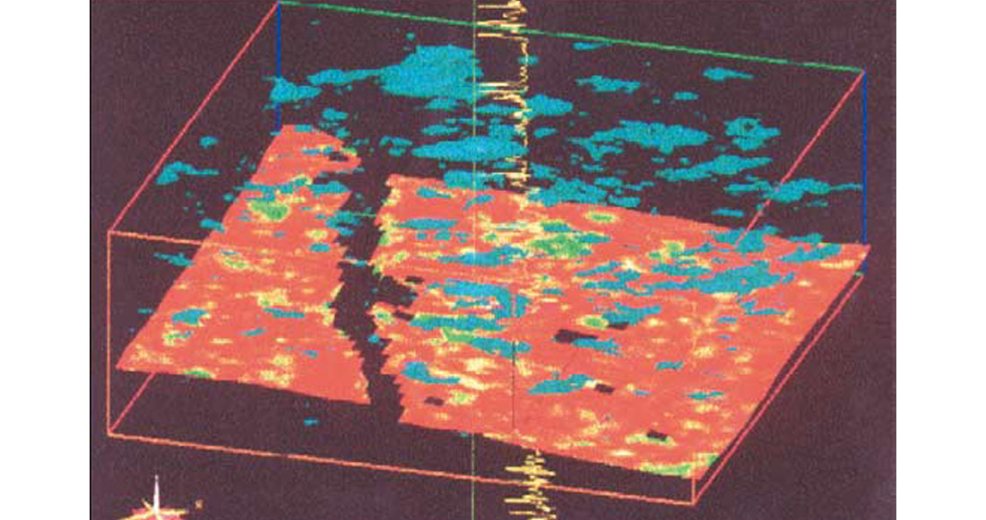
In geostatistical modelling, property and indicator (facies) simulations can be combined to produce both property (eg. impedance) and facies volumes. This is illustrated in Figure 7 from Torres-Verdin et al., 1999, which shows such an estimate from Argentinean data. The green patches are sand bodies from a single simulation. Favourable locations for new wells were determined by integrating the sand volume at each CMP for a set of simulations. The results of this development programme showed a definite improvement in sand detection. Accumulated production has been up to three times the field average in some instances, more than justifying the effort and expense of the inversion.

Important end results of 3D Geostatistical modelling are property probability volumes. A set of volume simulations of porosity, for example, can be modelled as a Normal probability density function at each grid point in time and space. From these, volumes can be constructed giving the probability that the porosity lies within a specified range. Figure 8 shows an example of this for simulations of porosity over a Western Canadian Devonian reef. Twenty simulations were used to generate a probability volume for the occurrence of porosity above 10%.

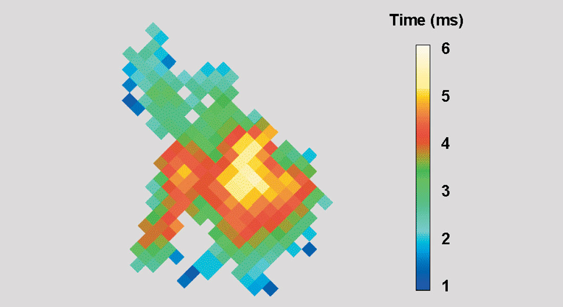
This volume was then viewed in 3D perspective and probabilities less than 80% were set to be transparent. The tops and bottoms of the viewable remainders were picked automatically. It is the thickness of one of these high-probability bodies which is mapped in Figure 8. The colours represent the thickness, within which, the probability of 10% or greater porosity exceeds 80%. In this way, uncertainty can be formally measured and input directly into risk management analyses.

Elastic Impedance Inversion

AVO analysis, which has been with us for many years, has taken a new and dramatic turn recently with the introduction of the concept of Elastic Inversion. Briefly, the thought process is as follows. We are familiar with the transformation of reflection coefficients to acoustic (zero incidence) impedance. Zoeppritz tells us that reflection coefficients are angle-dependent. What then would a transformation of angle-dependent reflection coefficients to impedance represent? We call this angle-dependent quantity Elastic Impedance and claim that an inversion of an angle or offset-limited stack would measure it. Such an approach addresses a whole host of problems including offset-dependent scaling, phase and tuning (Connolly, 1999). Both traditional AVO methods and Elastic methods which determine P and S reflectivities from seismic directly, do not deal with these issues correctly.

Simultaneous Zp, Zs Inversion

The elastic impedance inversion process can in fact be carried one step further with the simultaneous inversion of angle or offset- limited sub-stacks. This procedure brings all the benefits of inversion to bear upon problems encountered in traditional seismic weighted stacking approaches to AVO analysis. The outcomes are inversion volumes of P-impedance, S-impedance and density. Density is usually ill-defined and set to be constrained to the relationships observed in the logs.

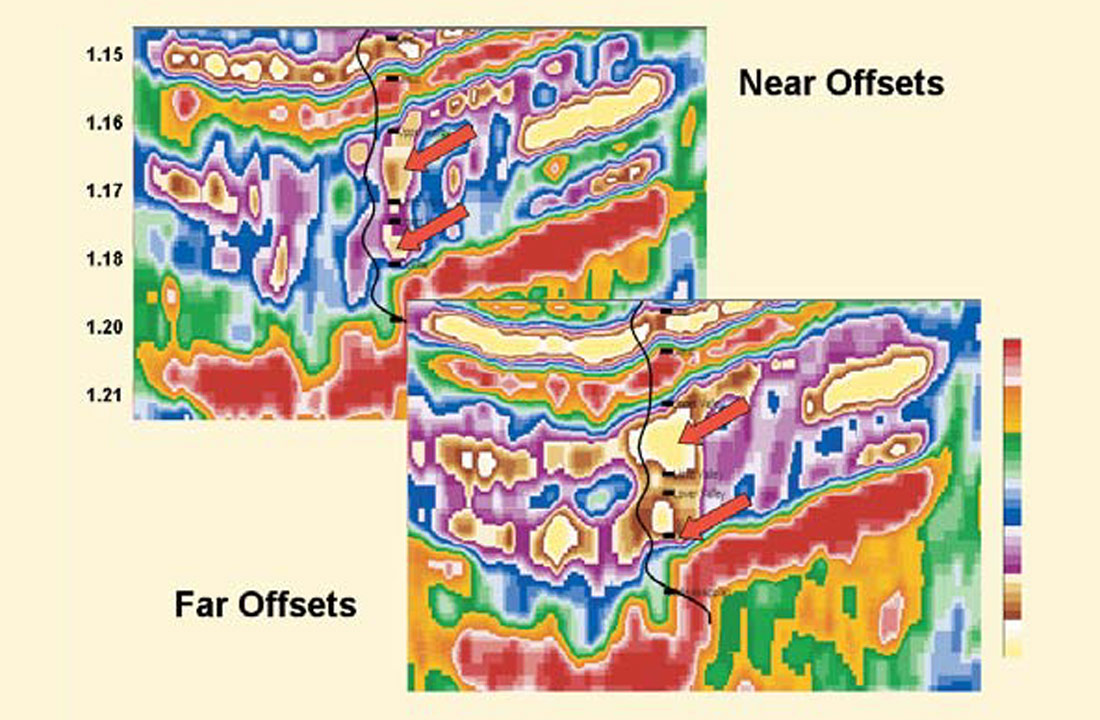
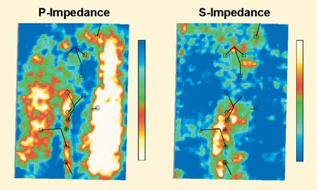
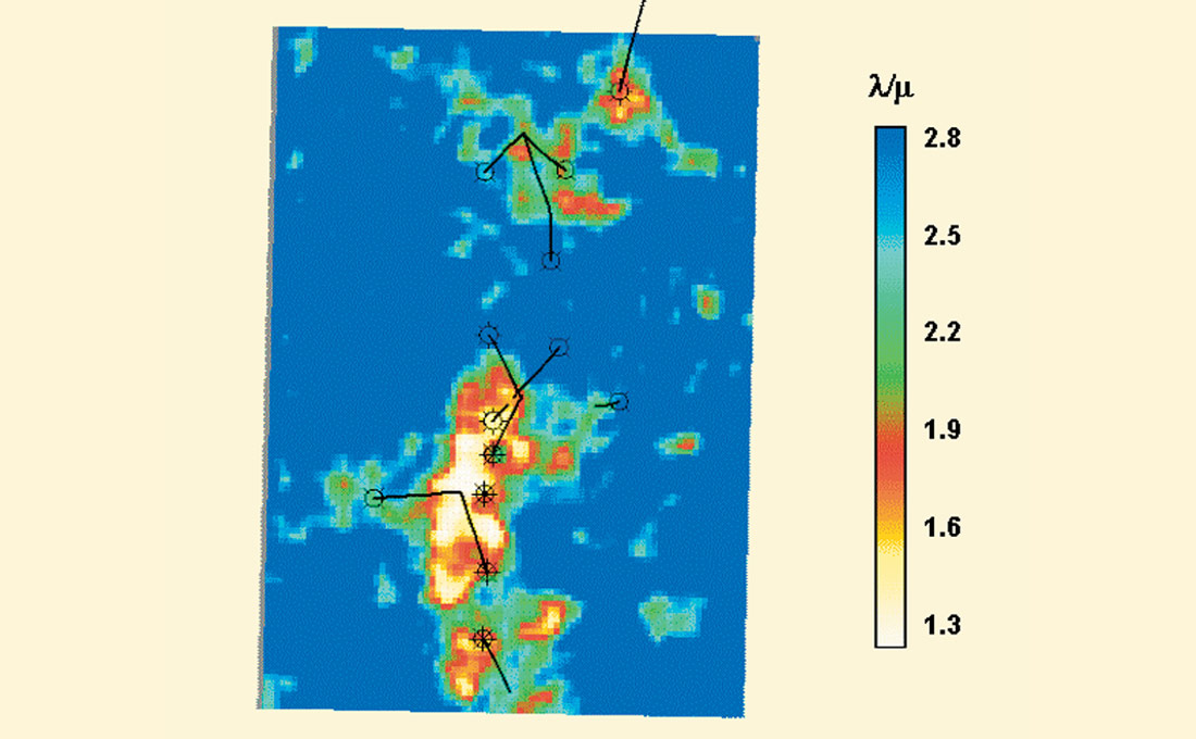
In Figure 9, we present an example from Pendrel et al., 2000. Detection of Cretaceous valley sands in the Blackfoot, Alberta area is problematic due to the similarity of their P impedance with that of shales. In Figure 9, the near and far offset stacks have been inverted separately. Note that the valley sands indicated by the arrows are softer (lower impedance) at the far offset. Figure 10 shows the results of the simultaneous inversion for the Upper Valley. The P-impedance is as much responsive to the off-valley shales as it is to the valley sands. The S-impedance section, on the other hand, highlights the highly-rigid valley sands. Transforming to the familiar Lame’ parameters LambdaRho and MuRho (Goodway et al., 1997), and then forming their ratio, results in a good sand discriminator (Figure 11).

Conclusions / Discussion

I hope in the above that we have conveyed the wide range of possibilities in modern seismic inversion and in particular those available through Jason Geosystems. Interpreters need to consider seismic inversion whenever interpretation is complicated by interference from nearby reflectors or the end result is to be a quantitative reservoir property such as porosity. Output in the format of geologic cross-sections of rock properties (as opposed to seismic reflection amplitudes) is endlessly useful as a means to put geologists, geophysicists, petrophysicists and engineers “on the same page”.

It is almost always useful to do sparse spike inversion first so that we may be crystal clear about what the seismic is telling us, free from bias from logs. These ideas are best expressed in the relative inversion. The absolute inversion brings in the logs as a geologic context for the relative inversion and at the same time, broadens the inversion band. Only after this, when the relation between the logs and the seismic has been ascertained should we consider methods, which make a stronger use of the logs. Model-based Inversion, Elastic Inversion, Simultaneous Zp, Zs Inversion and Geostatistical Inversion are all possibilities depending upon the data and the goals of the project.

I do not expect that the confusion over inversion nomenclature will disappear anytime soon. Perhaps, though, we have managed to shed some light on this topic. May I suggest that we reserve the term, model-based for those algorithms which, in a significant way, use logs to modify the inversion band within or above seismic frequencies?

The days of viewing seismic inversion as an extra processing step or subject of an isolated special study are long gone. Modern inversions are intimately connected to detailed and quantitative reservoir characterization and enhanced interpretation productivity. The process requires and integrates input from all members of the asset team. Horizons should be re-assessed, models re-built, log processing reviewed and inversion steps iterated toward the best result. After drilling, new information should be used to create a “living cube”, always up-to-date with all available information. It is this partnership directed to the solution of real reservoir characterization problems which leads to success.