Seismic Imaging: Post-Stack

Seismic imaging is a general term that geophysicists now use to describe processes that convert seismic data into a geological “representation” of the subsurface. These “representations” may vary from simple structural images that use migration algorithms, to ones that estimate rock properties with algorithms that are based on inversion theory. This first paper will address the basic concepts of modelling and poststack migration to build a foundation of knowledge for the following topic of prestack migration and seismic inversion.

The migration algorithms will be described by the three classifications of Kirchhoff, FK, and downward-continuation. To assist in describing these algorithms, a number of models will be presented that start with a known geological cross-section, which are then used to create seismic data. These models are then used to describe features of the migration algorithms.

Most of the material in this paper has been taken from my course notes that are published by the SEG. They contain an extensive list of references that have not been included in this review with the intent to keep it more readable. In addition, very little mathematics are used, which are replaced by basic physical principles that are used with the intention of providing a heuristic foundation of the migration principles.

Initial comments on depth and time migrations

In order to represent the geology of the subsurface, the final image “should” be viewed with a vertical axis in depth. However, many algorithms run much faster, and therefore much more economically, when the vertical axis of the migration is processed in time. These different processes are loosely referred to as depth and time migrations.

The objective of a depth migration is to position the reflected energy at its true reflecting geological location, and with an amplitude that represents the reflectivity at that location. In contrast, the objective of a time migration is to achieve the best focusing of the energy at a relative position. In structured areas, the relative lateral position deviates from the true lateral position by distances and times that may be estimated from image-rays that leave the surface in a vertical direction.

Depth migration requires considerable effort to build an accurate velocity model with axes of horizontal position and vertical depth. In some geological areas, errors in the location of the interface or in the velocity of shallow layers will cause errors in imaging deeper layers. Therefore, a number of iterations are required to build these depth velocity models, which usually commence by estimating the structure and velocities at shallower levels and then iterate to the deeper layers. Geological constraints should be continually applied during the development of the velocity model to ensure the structural integrity. At best, these depth migrations only produce an approximation to the subsurface with the actual horizontal and vertical positioning of reflectors being limited to some percentage of accuracy. However, in structurally complex areas, it may be too difficult to build an accurate depth model and time migration may be the only option to create a subsurface image.

Time migrations typically use a simpler velocity model with axes of horizontal position and vertical time. The velocity at a particular location may be used to focus energy at that location, and will be independent of the above or surrounding structure. A processor with limited geological input can construct these velocity models, with few iterations required.

The inclusion of anisotropic velocities has allowed more accurate velocity models to be constructed with accurate geological constraints, that may produce improved focusing and more accurate positioning of the migrated image.

Scatterpoint model and RMS velocities

Let’s assume that a small diameter buried pipeline P crosses a 2D seismic line at a right angle as illustrated in Figure 1a. This pipe will reflect energy from any source point on the surface to any receiver point on the surface although at this time we are only considering the energy that returns to a single receiver located at the source point. We refer to this type of reflector as a scatterpoint. Zero offset recordings are made at various locations across the surface, with their time response plotted below each surface location as illustrated in Figure 1b. The reflection energy lies on a curve defined by the two-way traveltime T.

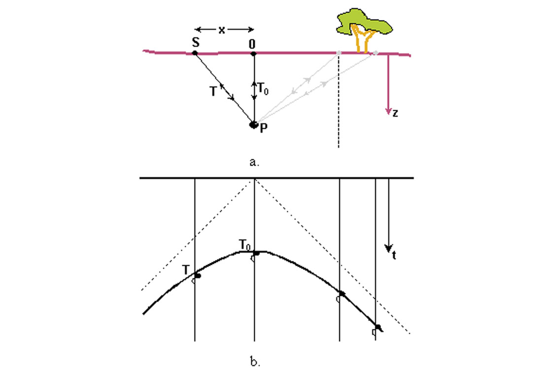
When the velocity of the subsurface is constant, the shape of the curve at time T is defined by the vertical traveltime T₀ from a source/receiver pair located immediately above the pipe at 0, and the distance x from location 0 to the location of a displaced source/receiver pair at S. Consider the triangle formed from the points (0, S, P) with two sides defined by T₀ and T. The third side has the distance x, which is converted (using velocity V) to a two-way time of 2x/V. With the units on the three sides of the triangle the same, Pythagoras theorem is then used to define the two-way travel time T by

The reflection curve defined is usually referred to as a “diffraction” with a shape that depends on the depth of the pipe (usually expressed by T₀) and the velocity V. The equation is exact for constant velocities, and is a very good approximation for horizontally layered media when the RMS velocity V_rms is used in place of V. In structured areas, the hyperbolic assumption may not be accurate enough and ray tracing or traveltime grids may be required to estimate the traveltimes.

When the displacement x becomes very large, T becomes proportional to 2x/V, defining a straight line that is referred to as an asymptote. These asymptotes are illustrated in Figure 1b by the dotted lines that intersect at the surface. All diffractions will have similar asymptotes that also intersect at the surface; a condition assumed by most migration algorithms. Therefore, changing the time datum before migration will prevent focusing data on a diffraction that is defined by equation (1.1), producing an inferior migration. Therefore, migration should be performed with time zero being as close to the surface as possible. Areas with rugged surface topography will require special attention.

Equation 1.1 is very important as it provides the basic traveltimes for many of seismic processes, including normal moveout correction (NMO), and most post and prestack time migrations that may include anisotropy and/or mode conversions. One-way traveltimes from the source to the scatterpoint, or from the scatterpoint to the receiver are computed by dividing this equation by two (2.0), leading to the double square root (DSR) equation, for prestack migration.

Diffraction modelling

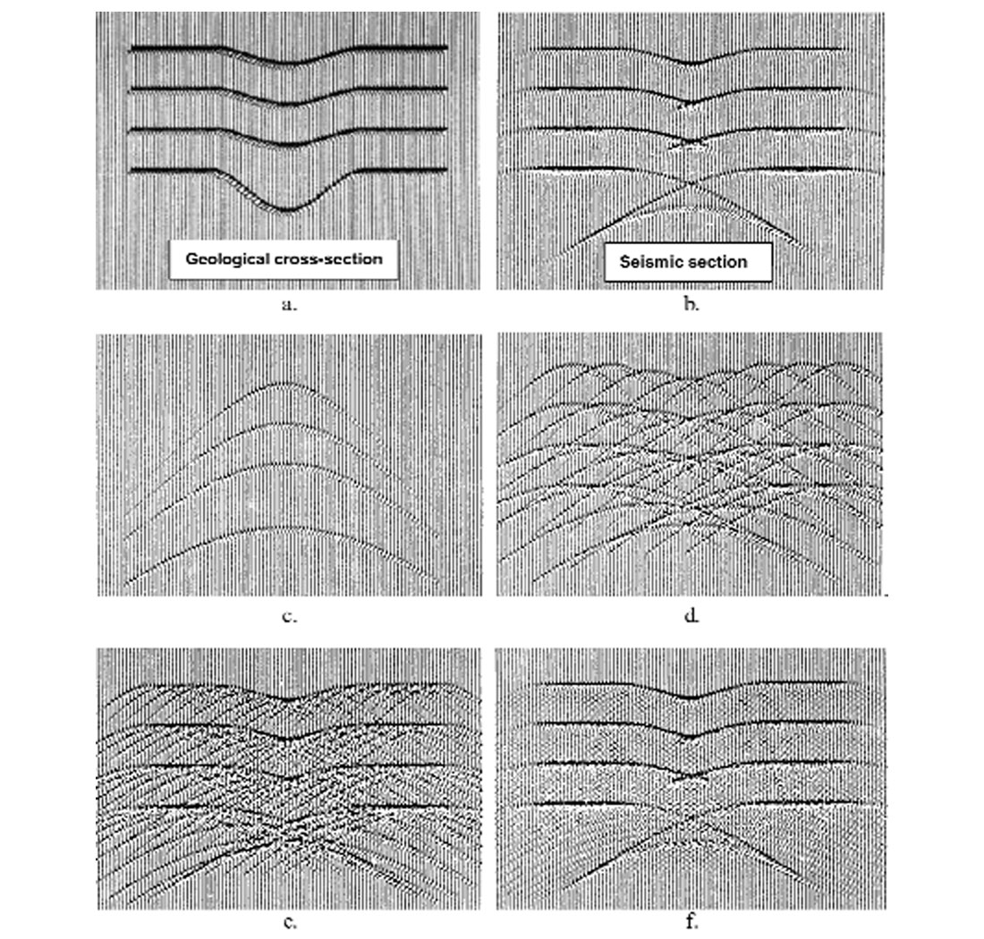
We extend the model described above to be more practical by assuming a reflector is composed of many scatterpoints, with each scatterpoint creating its own diffraction. It is usually sufficient to assume that the scatter points are located at equal increments along the reflector with spacing similar to the trace interval on the zero-offset section. To prevent aliasing, the wavelet is limited to a maximum frequency that depends on the velocity, dip, and trace spacing. This modelling technique is illustrated in Figure 2, in which four reflectors in the geological cross-section of (a) are modelled with diffractions to produce the section (b). In figure (c) only the diffractions from the center geological trace of (a) are shown. The number of geological traces used to create diffractions is increased to 8 in (d), 16 in (e), and 64 in (f). All geological traces are used in producing the completed zero offset section in (b). Note in (c), (d) and (e) that the diffractions are still identifiable, but in (f) their energy appears as noise. When all geological traces are converted to diffractions, as in (b), the noise cancels and the desired seismic model reconstructs.

The diffraction modelling technique is now used to imply that all seismic data are formed from diffractions. The reverse process of converting diffraction energy back to the geology may then be referred to as diffraction stacking or Kirchhoff migration.

Kirchhoff migration

Kirchhoff migration algorithms range from very simple time migrations to complex prestack depth migrations that can include anisotropy and or mode conversion. Three fundamental elements of all Kirchhoff migrations are

• the definition of a diffraction shape from a scatterpoint location,
• the summation of input energy along a path defined by the diffraction shape, and third;
• the placement of the weighted and summed value at the location defined by the scatter point.

This procedure is repeated for each sample in every migrated trace.

The kinematic shape of the diffraction may be assumed to be hyperbolic for a time migration, or a more complex shape that is defined by raytracing or the computation of traveltimes on a grid for a depth migration. Additional complexities occur when considering multiple paths to the scatter point, the existence of anisotropy, or varying propagation modes in elastic media.

Antialiasing filters may also be required to eliminate the inclusion of aliased input energy on the input data, operator aliasing of unaliased input data, or to prevent aliasing on the output section. Use of the antialiasing filters becomes a choice between the energy on dipping events, the presence of aliased noise, and computation speed. It should be noted that horizontal events have no aliased energy, but Kirchhoff migration can still introduce aliased noise when an antialiasing filter is not used as illustrated in Figure 4. The antialiasing filter is a zero-phase high cut filter that is uniquely defined by each point on the diffraction and can add considerable processing time to the algorithm. Consequently, a number of approximations to the filter are used, or it may even be eliminated.

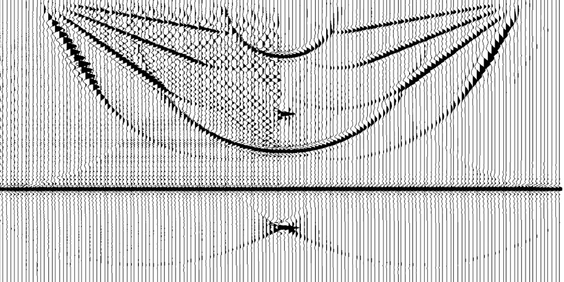
Figure 4 contains numerically model data that has been migrated on the left side without the antialiasing filter, while the right side includes the antialiasing filter. Note the presence of aliasing noise on the left side, even for the horizontal reflector (horizontal lines above the horizontal reflector). Also note that the steeper dip on the left side has a higher amplitude and higher frequency content (which happens to be aliased) than that of the corresponding dip on the right side.

To this point we have only stated that we sum the energy within the diffraction window, which leads to the term, “diffraction stack method”. Could we get a better image if each input sample, defined by the diffraction, was weighted by a unique value chosen from a weighting function? This dilemma was resolved when it was recognized that the diffraction stack method was similar to a Kirchhoff integral solution to the wave equation that was used in optics. This integral solution to the wave equation provided an amplitude scaling and phase shifting term that improved the focusing of the diffraction stack migration, which we now refer to as Kirchhoff migration. The relative amplitudes of the weighting function may be simply defined by T₀ / T, defined as being proportional to the length of the raypath, computed using the transport equation, or computed by multipath raytracing. (The amplitude weighting of prestack Kirchhoff migration is a very complex issue and is typically the topic of various solutions to the inversion problem.)

One of the main advantages of Kirchhoff migration is its ability to use arbitrary input or output geometry. Figure 3 illustrated that one output sample could be migrated. (This is in contrast to the other methods that require all the input data to produce all the migrated data.) This arbitrary geometry feature enables small subsets of data to be migrated very rapidly, such as a “porthole,” which could be a small window of migrated data that is limited to small ranges of traces and depths (or times) from either 2D or 3D data. Other subsets of data could be the migration of all input 3D data to an arbitrarily located 2D line, or to any defined time-slice (or depth-slice).

The arbitrary geometry property of Kirchhoff migration also allows 3D data that is acquired with a bin spacing of 25m by 50m to be migrated to a new bin spacing of 20m by 20m. In addition, a number of input 3D projects with different acquisition geometries and layout directions can be efficiently combined into one migrated volume without a prior interpolation to the new migrated grid.

The migration aperture is often defined as a spatial distance that limits the range of input traces that are migrated to one output location. While this definition may also be used for Kirchhoff migration, it should be noted that the lateral extent of the summation window could be limited for each migrated sample. This is usually accomplished by a dip limit that is placed on the diffraction. For a given dip limit, the lateral extent of the diffraction will be small for shallow data and large for deeper data. Within this context, the migration aperture of a Kirchhoff migration may be considered to be time variant.

FK migration

Use of the Fourier transform can greatly simplify the migration process as illustrated in Figure 5. An input 2D zero offset section p(x, t) in (a) contains three events with dip α. This input section is 2D Fourier transformed into P(K_x,ω) in part (b) where wavenumber Kx is the Fourier transform of the x component, and radial frequency ω the Fourier transform of the t component (often written as frequency F; giving the name “FK” migration). All energy with the same dip is aligned together in the P(K_x,ω) domain with the dip a measured from the vertical. We now make a quick visit to the wave equation, which is expressed in the time-space domain in equation (1.2) and in the wavenumber-frequency domain in equation (1.3). Note that equation (1.3) contains three squared terms that could (and do) represent the sides of a right-angle triangle

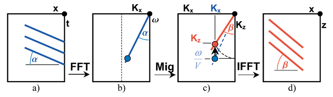
Solving equation (1.3) for K_z we get equation (1.4), which quantifies the data movement in Figure 5c in which a sample of energy located at P(K_x , ω/v) with dip α before migration, is moved vertically to location P(K_x , K_z) with dip β after migration. After the data movement the point P(K_x , K_z) defines a triangle where the radial distance is given by ω/v, according to equations (1.3) and (1.4). Thus, the migration algorithm in the frequency domain is a simple point-to-point data movement, which is very fast relative to the other algorithms and is an efficient means of applying the migrator’s equation, tan α = sin β, in the frequency-wavenumber domain. The inverse 2D Fourier transform produces the migrated section P(x, z) with the three events at dip β.

Unfortunately, the temporal and spatial locations are not easily identified in the transformed space and the process assumes a constant velocity. This restriction is partially overcome by performing a vertical time-to-depth stretch (really a variable to constant-velocity stretch) prior to the initial transform and a corresponding depth-to-time conversion after the inverse transform. The time-to-depth stretch requires a velocity field in which the average or RMS velocities have been smoothed. Consequently, the FK migration algorithm may be used successfully in areas with smooth velocity variations such as the marine environment, sedimentary basins, or the exposed basement for mining in granite. In these areas, the inclusion of dip moveout (DMO) is also recommended.

One effect of the time to depth stretch is to reduce the effects of lateral velocity variations, producing a migrated section that tends to locate migrated energy closer to the lateral position of a depth migration.

Even though FK migration is only ideal for constant velocity data, it does have a number of additional applications that make use of it speed and accuracy. Some migration procedures migrate the input section a number of times at different constant velocities and then form the final migrated section using a cut-and-paste method that selects the output according to the velocity model. Another application cascades two different migration algorithms in which the steep dip feature of the FK algorithm is combined with a shallow dip algorithm that uses variable velocities. In this case the first stage is a constant velocity FK migration, which then becomes the input to the second stage in which the variable velocity migration algorithm is performed using a modified velocity field. The FK algorithm also provides an ideal solution for comparison with the solutions from other migration algorithms that are tested with a constant velocity. Any differences may be attributed to the algorithm under test.

The Fourier transform may also be used in some Kirchhoff migration algorithms where accurate time shifts are computed with linear phase shifts, or in the downward continuation process where one depth layer is extrapolated to the next depth layer.

Downward continuation migration

Modelling seismic data at varying depths

The left side of Figure 6 contains four simple constant-velocity geological structures (a), (c), (e), and (g), that have varying surface elevations, and one scatterpoint at a fixed elevation. The right side of the figure contains the corresponding zero offset seismic sections (b), (d), (f), and (h), with time zero located adjacent to the recording elevation. As the depth to the scatterpoint is decreased, the time to the apex of the diffraction is also decreased. The extent of the diffraction is limited to the same dip and becomes smaller as the recording surface moves down toward the scatter point. At the fourth level, when the recording surface is at the depth of the scatterpoint, the reflected energy in the diffraction is concentrated at the location of the scatter point. In a real recording situation, this recorded amplitude would be very large and distorted, but it is still a useful exercise to contemplate.

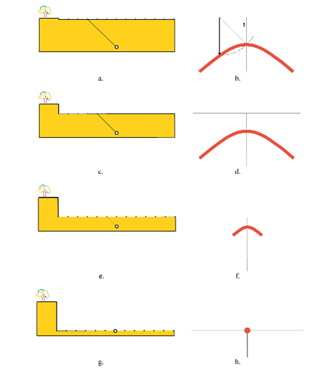
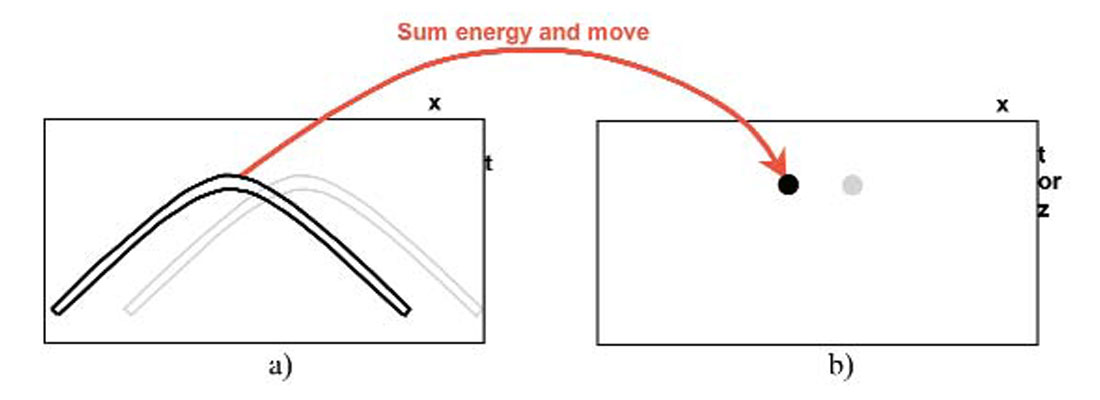
Now consider the same content of Figure 6, however assume that energy contained in the lower three seismic sections (d), (f) and (h), is somehow computed from the shallower section. Each section now corresponds to a recording at a given depth (or elevation). In each case, the diffraction is raised in the time section and the extent of the diffraction reduced, however the total energy in the diffraction remains the same. In the last section (h), all the energy is concentrated at time equal to zero. Note that the depth of this section (h) corresponds to the depth of the scatter point. This method of propagating the seismic sections to increasing depths is referred to as downward continuation migration, and energy that focuses at time zero is mapped to the migrated depth section at that depth.

Downward continuation migration

The downward continuation method of migration is also illustrated in Figure 7, where the seismic sections from Figure 6 are now arranged in a cubic form V(x, z, t) with each time section located at the corresponding recording depth z. The input 2D section p(x, t) is the top surface of the cube V(x, z=0, t) and identified by the blue outline in Figure 7. The increments in depth are identified by δz in the depth migration of (a). The energy from the diffraction at z = 0 is now focused in the direction of the brown dashed line to a point at time t = 0, on the fourth depth level (z=3 ▪ δz), corresponding to the section in Figure 6h. When all layers of the volume have been computed, all other diffraction on the input time section would be collapsed to their corresponding scatterpoints on the depth migrated output section V(x, z, t=0), identified by the brown outline in Figure 7a.

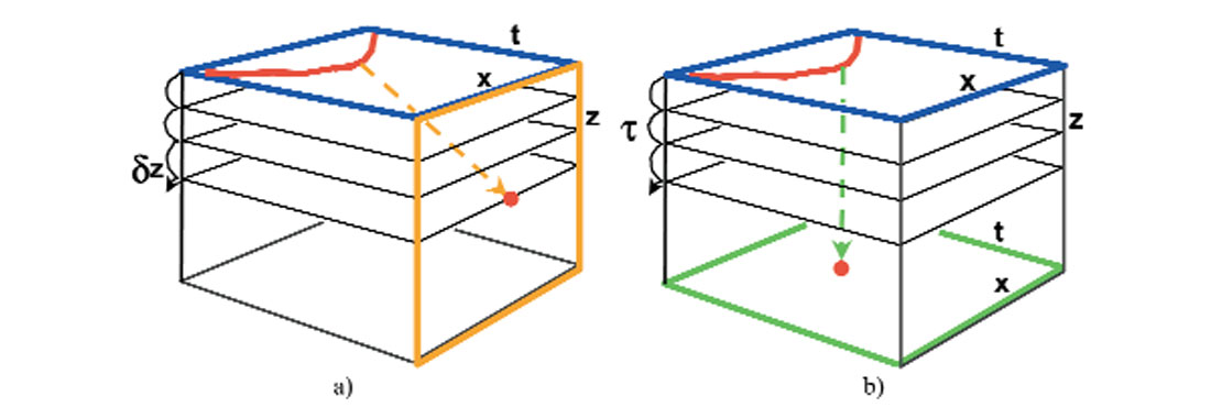
The downward continuation algorithm could be modified to prevent the diffraction rising in time, enabling it to collapse toward the same location at the apex of the diffraction as identified by the green dashed line in Figure 7b. At the appropriate depth level, z=3 ▪ δz, or corresponding time increment 3 ▪ τ, the energy has focused to the peak of the diffraction, and that portion of focused data is mapped to the bottom of the volume. When the entire volume is computed, the output is a time migration identified by the green outline of V(x, z=z_max, t).

Exploding reflector model

The final model to be introduced is the exploding reflector model (invented by the late Dan Loewenthal) that identifies how energy can be propagated from one depth level to the next. This model replaces the two-way raypaths from the colocated source and receiver, with a single raypath (at half the velocity) from the reflector to the surface. This model assumes that the source point for each ray is located on the reflector, and leaves with a path normal to the reflector at time zero. The model becomes more general when we consider each point on the reflector to be a scatter point that radiates energy in all directions creating a diffraction pattern when recorded on the surface. When considering all the source points on the reflector, it would appear that the entire reflector exploded at time zero. At a fixed interval of time, all the exploding points would construct a wavefront corresponding to that produced by the exploding reflector as illustrated in Figure 8.

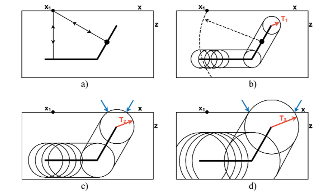
Figure 8a shows two two-way raypaths for a source and receiver located at x₁. A seismic trace recorded at x₁ will contain energy at the corresponding traveltime. In contrast the circles in Figures 8b-8c represent some of the wavefronts from exploded scatterpoints on the reflector at the specific times of T₁, T₂, and T₃. The summation of all scatterpoint wavefronts would reconstruct the wavefront of the exploded reflector. At time T₂, some energy has propagated to the surface at z = 0, as indicated by the blue arrows and is recorded on the seismic traces at that location x, and at that given time T2. At the later time T₃, the wavefront has expanded to new surface locations as indicated in (d). If the wave fronts were computed at two millisecond intervals, then the sample in all the seismic traces would be samples at two millisecond intervals.

The dipping reflection point in Figure 8a is also shown in (b) along with its wavefront (dashed curve) at the same two-way time of the raypath. The wavefronts from all scatterpoints on the dipping event would construct a single wavefront that passes through the same point x₁ with a kinematic response that is identical to that of the raypath in (a).

A collection of all the geological cross-sections, in which the wavefronts have been computed at equal increments of time, are arranged in a cubic form with dimensions V(x, z, t) as illustrated in Figure 9a. The geological structure is viewed on the front surface V(x, z, t=0) with subsequent images on planes with constant time ti V(x, z, t=t_i). The resulting seismic section is the top surface V(x, z = 0, t).

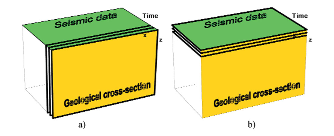
The energy on each geological cross-section can be computed from the previous cross-section by using various solutions to the wave equation. For example, energy at time zero V(x, z, t = 0) can be propagated to the next time increment at increment V(x, z, dt) and then to V(x, z, 2 dt) until the entire volume is computed.

Now consider the reverse process. Using the same model of the exploding reflector, we could start with seismic data on the top surface of the volume, and using the wave equation, propagate the energy back into the subsurface, in a downward manner, as indicated by the depth slices in Figure 9b. The front surface V(x, z, t=0) would then represent the geological cross-section or depth migration.

When using the wave equation to move energy from one depth level to the next, it is convenient to start with the Fourier transform of the wave equation and find the derivative of the wavefield in the depth or z direction, i.e. equation becomes

Exact solutions of this form lead to the phase shift method of Gazdag, or the combination method of Margrave. The square-root part of equation (1.5) may be expressed as a power series in the form

Truncation or simplification of the power series leads to many approximate solutions, which may be converted back to the time-distance domain and used in the finite-difference method. For example, using the first two terms of the power series leads to the 15-degree finite-difference solution. Other finite-difference solutions with more accurate approximations to the square-root are referred to as the 45°, 60°, and 65° solutions, indicating their relative accuracy to increasing geological dips. Other algorithms such as the finite difference ωX, make use of the Fourier transform to increase the accuracy of the computation.

The phase shift method uses equation (1.5) in its exact form and is repeated with an extra term as

Note that the coefficient a on the right side of the equation is independent of z (assuming V is constant at this depth z), and that the solution to this equation is the exponential function

Adding a dz to the depth z in this equation we get

or with all variables,

Equation (1.10) informs us that propagating energy on the z layer to the next layer at z + dz is easily accomplished in the frequency-wavenumber transform domain by multiplying each point by a constant, and that the constant is an exponential term or a complex number with unit amplitude.

The method is theoretically accurate when a constant velocity is used for each extrapolation step. However, the velocity may vary for each depth increment allowing a theoretically accurate migration when the velocities vary only with depth. Approximations to the phase shift method such as phase shift plus interpolation (PSPI) interpolate a new depth increment from a number of constant velocity extrapolations, which then allow the velocity to vary both laterally in x and vertically in z. The theory of the phase shift method may also be used in an ωX method that extrapolates a surface in which the wave number is transformed back to distance x, for a volume V(x, z, ω), enabling velocities that vary in both x and z.

Resolution

In the early 1980’s many processing supervisors were reluctant to use migration on data that contained flat events, due mainly to the expense. They correctly assumed that perfectly flat events should not change after migration, but did not recognize that events that appeared to be flat could actually contain anomalous structure. Fortunately, it was recognized that events on a stacked section have a horizontal resolution that is described by the Fresnel zone, and that anomalies contained within horizontal events that contain anomalies are spatially smeared and may not be visible. Migration collapses these Fresnel zones, leaving the spatial resolution to be theoretically the same as the temporal resolution. However, practical limitations such as the aperture of the diffractions or the approximations used in the migration algorithm do reduce the spatial (or orthogonal) resolution.

Conclusions and comments

All migration methods are based on various solutions to the wave equation. The Kirchhoff method is an integral solution to the wave equation, while the FK method makes use of the Fourier transform. The downward continuation method utilizes a number of techniques to solve the wave equation such as the finite difference method or the phase shift method.

The principles of poststack migration have been applied by the seismic industry in various forms for the last fifty years and will continue for a number of years to come. These poststack migrations operate on a stacked section that is assumed to have zero offset. However, the process of stacking common midpoint gathers is only valid for horizontally layered media. Data that contains dips or truncated events will not stack all the reflected energy to the correct zero offset location. It is prestack migration that eliminates conventional stacking and enables all energy to be focused correctly.

In the early 1980’s, considerable effort was required to convince the industry that migration was necessary, especially for flat data. Today, the same effort is required to convince the industry that prestack migration is necessary, especially for flat data. This topic will be discussed in the next paper of this series, “Review of seismic imaging: prestack”.