Seismic Detection and Estimation of Overpressures Part II: Field Applications

Summary

Subsurface formations with pore fluid pressure in excess of the hydrostatic pressure (geopressure) are encountered worldwide. Although there are a multitude of causes that can result in geopressure, under compaction due to rapid burial of sediments is the predominant cause of geopressure. Typically, if the loading process is rapid, fluid expulsion through compaction is severely retarded, especially in fine-grained sediments with low permeability such as silts or clays. This results in stress redistribution within the column - a greater proportion of the overlying weight of the sediments is borne by the fluids than when the sediments compact normally, causing a decrease in the stress acting on the rock framework. Dehydrating bound water from clays within shales further complicates this phenomenon as compaction proceeds with the depth of burial with increase in temperature.

Geopressured formations pose significant threats to drilling safety, and the cost of mitigation, especially, in deepwater settings, is high, to the tune of $1.08 billion per year world-wide. Proper planning before drilling is key to lowering costs and increasing safety. In this regard, the role of seismic is of paramount importance. Seismic wave attributes (amplitude, velocity, coherency, etc.) are affected when stresses acting on the sedimentary column (effective or differential stress) are low. These attributes can be analyzed to obtain signatures of overpressure or lack of fluid transport over the geologic time- both qualitatively and quantitatively. Using the seismic signatures, zones of trapped fluids and pressured compartments can also be mapped prior to drilling. With either an analogue or a reliable low-frequency velocity model, it is also possible to map fluid transport effects in the reservoir scale using seismic inversion techniques.

In this paper, we illustrate how this process works using seismic data at various scales, from the low frequency reflection seismic at exploration frequency scales to those employed at well-logging scales. A rock-model-based approach especially suited for deepwater pore pressure imaging is introduced. It includes the effect of shale burial diagenesis, and uses the velocities derived from inversion of prestack seismic data. The procedure yields details of pre-drill pore pressure images with significant clarity as well as pressure versus depth profiles appropriate for drilling applications. In particular, prestack full waveform inversion yields Poisson’s ratios that are useful not only for pressure and fracture gradient estimations but also for lithology and fluid identification. This technique is also applicable to identification of shallow water flow formations that pose drilling hazards in deep water. The procedure is illustrated with examples from several deep water basins.

Introduction

It has been a common practice to predict pore pressure before drilling from the conventional seismic stacking velocities with a normal compaction trend analysis using, for example, the well-known Eaton approach (Eaton, 1972). Velocities that appear to be slower than the ‘normal’ velocities are indicative of overpressure, which then is quantified using an empirical equation. There are several problems with this approach. First, the conventional seismic stacking velocities are usually unsuitable for pressure prediction since they are not “rock or propagation velocities” (Al-Chalabi, 1994). Second, these velocities lack resolution in depth. Third, in a deepwater environment, sediment loading has often been so fast that pressures in these sediments are above hydrostatic (geopressured) right below the mud line – unlike, for example, on the continental shelf of the Gulf of Mexico (Dutta, 1997). This prevents development of a normal compaction trend, thus invalidating the entire approach in the deepwater. Even when a velocity trend is constructed (with depth as a variable) by curve-fitting pressure data from an analogue well, most of these trends violate the fundamental bounds of rock physics: the velocity neither approaches the correct sediment velocity just below the mudline nor approaches a limiting velocity appropriate for very low porosity rocks at very high overburden pressure.

The approach discussed here and in Part 1 (Mukerji et al 2002) is trendline- independent as it uses a rock model for geopressure analysis, namely, effective stress as a function of lithology, porosity, velocity, and temperature, to name a few. This model then drives the interpretation of seismic data. The input data are based on analysis of several seismic attributes, such as velocities and amplitudes, and are calibrated with offset well information. Pore pressure is calculated as the difference between overburden stress and effective stress. The effective stress affects the grain-to-grain contacts and consequently, the velocities of seismic waves propagating through the rock (Domenico, 1984; Dutta, 1997). The rock model used in the present work is based on the general rock physics principles discussed in Part 1 (Mukerji et al 2002). It has several components: relations between porosity, lithology and velocity, clay dehydration (which is a function of clay type and its burial history), and transformations relating both the density and the Poisson’s ratios of the sediments to the effective stresses acting on the matrix framework. The key inputs that drive the rock model are velocities and amplitudes of P and S waves obtained from a variety of seismic tools (discussed below). Iterative velocity calibration and interpretation are two essential steps in the prediction process to ensure that the velocity fields are within the realm of expected rock or propagation velocities.

Role of Rock Model in Pore Pressure Imaging

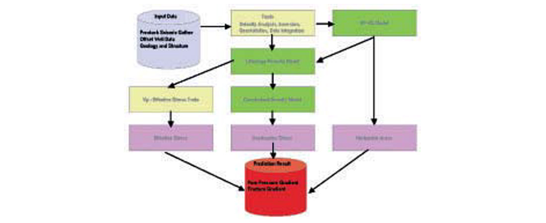
Dutta (1987) discussed causes of overpressure and various ways to detect such a phenomenon. Seismic imaging has been a key tool that provides estimates of subsurface pore pressure prior to drilling. Figure 1 shows the key steps in pressure prediction using seismic data. The steps involve:

• Assessing the cause of overpressure (compaction and clay dehydration, for example)
• Developing a rock model for relating rock attributes (velocity, porosity, Poisson’s ratio, for example) to higher-than-normal pore pressure or lower-than-normal effective or differential pressure (which is the stress acting on the rock matrix)
• Using a fit-for-purpose seismic velocity that resembles rock velocity and not processing velocity as stated very clearly by Al-Chalabi (1994).

Pore fluid does not support shear-wave propagation, and poor grain-to-grain contacts in the overpressured zones with low effective stress affect the S-velocity even more than the P-velocity. This has been observed in the laboratory (Domenico, 1984) and modeled (Xu and Keys, 1999; Zimmer et al 2002; Mukerji et al., 2002). The Vp/Vs ratio (which is directly related to Poisson’s ratio) is a key parameter that relates to low effective pressure or high pore pressure, especially under the SWF conditions (pore pressure close to fracture pressure). This has not received much consideration in pore pressure prediction methodologies, mainly because the traditional seismic approach for pressure prediction used the conventional P-velocity data only.

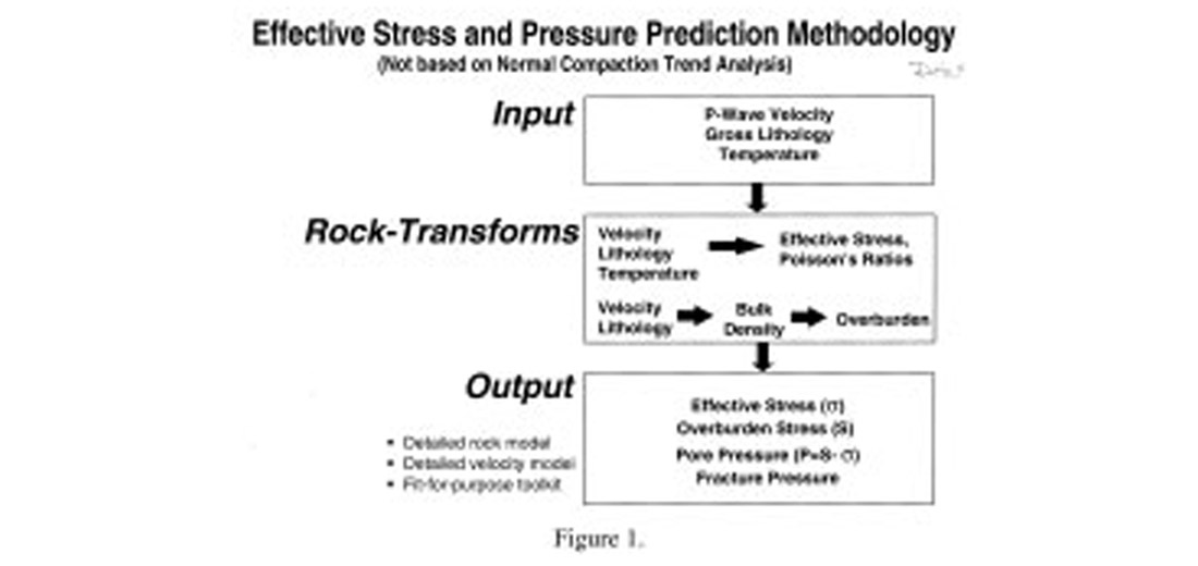
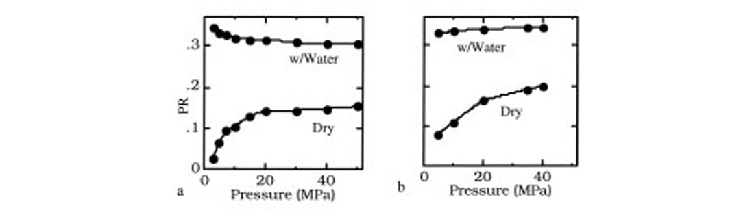
Figure 2 shows a plot of Poisson’s ratio (PR) versus effective stress based on the data from Stanford Rock Physics laboratory for two cases: sand filled with water and sand filled with gas. Note the behavior of Poisson’s ratio at low effective stress. For the water-filled case, the ratio increases with increasing pressure (lowering effective stress), whereas the opposite is true for the gas-filled case. The increase of the saturated-rock PR with increasing pore pressure has a physical basis. The higher the pore pressure, the softer the rock and the larger the relative increase in the bulk modulus between dry and water-saturated samples. With the shear modulus being the same for the dry and saturated rock (Gassmann, 1951), PR is larger in the saturated than in the dry sample, especially in soft rocks. An example of the saturated-rock PR increasing with decreasing differential pressure is given in Figure 2a. However, one may observe the opposite effect as well (Figure 2b). The direction of the saturated-rock PR change depends on the porosity and elastic moduli of the sample and has to be calibrated by using fluid substitution with site-specific rock data.

The difference in the dry and saturated PR vs. effective stress suggests a very different seismic signature for the two cases in the amplitude-versus-offset (AVO) domain. Modern pore pressure prediction methods exploit this fact by inverting CMP gathers using the full waveform inversion technology (see below) that allows extraction of the Vp/Vs ratio from large offset P-wave data (Mallick and Dutta, 2002-TLE; Dutta, 2002- TLE). Miley and Kessinger (1999) demonstrated how to use this effect on shear velocities that were determined from mode converted wave reflections for subsalt pore pressure prediction.

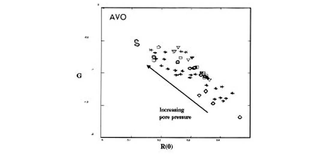
Figure 3 connects measured rock properties to seismically derivable attributes. In Figure 3 we see P-to-P AVO attributes, zero-offset reflectivity [R(0)] and gradient (G), computed from Gulf of Mexico sandstone data for different effective pressures (Takahashi, 2000). The attributes were calculated using Shuey’s approximation for angle-dependent P-to-P reflectivity, from measured values of core V_P, V_S, and density, with average properties for the shale caprock. The arrow shows the trend of change in AVO behavior with increasing pore pressure or equivalently, decreasing effective pressure.

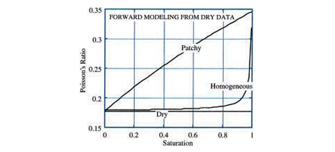
It has become recognized that gas saturation can dramatically influence seismic velocities and Poisson’s ratio, and hence AVO patterns in overpressured soft sediments. However, what is not so well known is that it is not only the amount of saturation, but also the spatial distribution and scale of saturation—homogeneous versus patchy—that can greatly affect the seismic response. In homogeneous saturation gas is finely mixed with oil or brine, and is uniformly distributed within the pore space. For a patchy or heterogeneous saturation distribution, fully-saturated patches of oil and brine are surrounded by dry, gas-filled regions. The difference in the Poisson’s ratio between these two saturation scenarios can be dramatic (Figure 4). This difference can give rise to distinct AVO patterns that can be used for seismic overpressure detection.

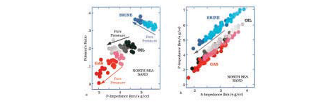
P-wave impedance and Poisson’s ratio can be obtained from seismic data using acoustic and elastic impedance inversion (e.g., Connolly, 1998). It is, therefore, important to create diagnostic rock physics based charts that will help interpret the inversion results in terms of pore pressure and pore fluid. An example of diagnostic charts is given in Figure 5, based on laboratory measurements of the elastic-wave velocity in unconsolidated North Sea sands (Blangy, 1992). Different regions in the PR versus P-wave impedance plane and P-impedance versus S-impedance plane correspond to different pore pressure and pore fluid. One can identify both pore pressure and pore fluid from seismic (and separate the pore pressure effect from the pore fluid effect) by superimposing seismic elastic rock properties on a diagnostic chart. Such plots, calibrated to specific locations and lithologies of interest, can guide us in looking for anomalies in seismic attributes that might indicate overpressures.

Velocity Analysis

Velocity and amplitudes are two key attributes that relate to pore pressure imaging (PPI). Figure 6 describes the general process flow for PPI. The main features of the process flow are:

1. Model-based approach for geopressure prediction.
2. Inclusion of multiple geopressure mechanisms (compaction, shale burial diagenesis).
3. A methodology that does not require the normal shale compaction trend analysis
4. The method is applicable to zones of very low effective stresses (hard pressure, for example)
5. Use of special handling of seismic velocities for geopressure analysis (extracting rock velocity from seismic velocity using fit-for-purpose velocity analysis tools).

Processed seismic data are used to derive a 3D velocity field appropriate for pore pressure estimation. In a recent paper, Dutta (2002) discussed various seismic velocity tools that can be used for pore pressure evaluation. Velocity analysis (VA) is performed using prestack processed gathers from every CMP’s for better lateral continuity. Below we provide a very brief description of various velocity analysis tools that we have used for PPI with considerable success. For more details we refer to Dutta (2002).

Semblance velocity analysis

Interval velocity functions are interpreted using semblance displays, in both time and depth. A suite of supplementary information is available at each CMP location, including horizon times, neighboring functions, velocity fans, histograms, proximity velocity overlays, log overlays, and model functions. To further aid the interpretation, a CMP gather, a multiple velocity function (MVF) stack panel, and an interactive stack panel are available. All the processes invoked at a particular CMP location are fully integrated. A key step in the velocity analysis is to use rock physics to constrain the interval velocities so that the velocities are meaningful and without spikes— the features that invalidate any routine use of stacking velocities for PPI. A key step, therefore, is to interpret and QC velocities using a velocity template for pore pressure analysis.

Spatially continuous velocity analysis and automated velocity model building

Automated Velocity Model Building (AVMB) is a process to automatically generate and update high-resolution 2D and 3D interval velocity models using migrated seismic data (Mao and Deregowski, 1999). AVMB employs an automated velocity picker, Spatially Continuous Velocity Analysis (SCVA), to generate continuous time-velocity pairs at every CMP location and for every time sample. A constrained least-squares regression is used to generate the interval velocities that best match the observed stacking velocities. Lateral cascaded median smoothing is used to preserve any lateral velocity discontinuities within the data according to user specified resolution criteria. The detailed interval velocity field generated by this process is utilized for pressure imaging after quality control by human intervention at key steps, such as assessing the impact of multiples on the velocity model.

Tomography and Prestack Depth Migration

For complex geologic environments where ray path bending is important, we use various tomographic and migration velocity analysis. Again, these velocities are conditioned to comply with what is expected from a rock-physics-based model, as highlighted above. Both layer- and grid-based tomographic tools are used, depending on the complexity of the geology. When properly conditioned, tomographic velocity inversion will provide a laterally extensive and reliable image of the velocity field, which will approximate the 3-D rock velocities more closely.

A review of the literature suggests that the velocity inversion approach is very useful in the cases where velocity contrasts in subsurface rocks are sizable. Examples are Clastics overlaid by carbonates, shallow gas layers or pockets, and very high overpressures. Quite often, we see a remarkable improvement in the quality of the tomographic image over that obtained using Dix’s interval velocities. However, the technique sometimes misses subtle changes in the velocity fields due to the limited bandwidth of reflection seismic data.

Prestack depth migration has been proven to be an excellent tool to provide a clear picture of targets in areas like sub-salt or sub-basalt. However, these velocities are created with one goal in mind, ‘focus the image’. This is not necessarily good for pore pressure analysis. Typically, image gather velocities are too high, and thus pressures are too low. To avoid this problem, we convert the CMP gathers in time and re-pick the velocities in time domain as discussed by Al-Chalabi (1994). Further, rock-physics-based constraints are also used to condition the interval velocities.

The methods of seismic reflection tomography and migration may be viewed as complementary processes. Migration requires velocities in order to image reflector boundaries, whereas reflection tomography requires reflector positions to estimate velocities. However, it is for this reason, that the tomography-derived velocities are more appropriate for pressure analysis than those from the straightforward depth imaging process.

In summary, one must use a fit-for-purpose tool-kit for velocity analysis for pore pressure imaging. The goal is to derive velocities that are close to rock velocities—the ones that are related to effective stress and pore pressure. The key steps in the process involve the velocity analysis that includes residual NMO correction, higher order moveout effects, analysis of velocity anomalies, anisotropy correction, and velocity interpretation to honor the local geology. Further, for laterally varying geologic environments, velocities based on tomographic inversion and migration are required for pressure analysis.

Anisotropy Correction

The subject of seismic anisotropy is complex and a detailed discussion of that in the present paper is beyond the scope. However, anisotropy corrections to seismic velocity analysis impact predicted pore pressures from seismic velocities in an important way – it increases the predicted pressures. This is because, for predictive purposes, one needs the vertical or well velocity. However, the seismic velocity analyses discussed above yield velocity functions that are mostly horizontally propagating. This velocity function will therefore be faster than the well velocity function; and hence, the predicted pressures, without accounting for anisotropy, will be lower.

In many basins around the world, sedimentary rocks can be simplified as a vertically transversely isotropic (VTI) medium. For such a medium, wave travels vertically and horizontally with different velocities, e.g., Vo (vertical velocity) and Vh (horizontal velocity). As noted above, velocities from normal moveout (NMO) analysis are usually higher than those from wells due to the fact that NMO analysis measures the wavefront curvature at a near vertical angle, which is distorted by anisotropy parameterized by ellipticity parameter d and an ellipticity parameter h, whereas the measurement from well gives the vertical velocity of a rock matrix. Thomsen (1986) showed that NMO velocity from moveout analysis is neither vertical velocity nor horizontal velocity and characterized the effect of anisotropy on wave propagation by introducing three parameters, ε, η and δ. Yang et al (2002) used Thomsen’s weak anisotropy concept and showed how to correct for it using an extended moveout analysis.

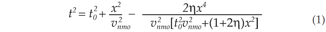
The procedure can be described briefly as follows. The starting point is the anisotropic moveout equation for a weak VTI medium as described by Alkhalifah and Tsvankin (1995),

For practical purpose, Yang et al. (2002) define two ratios as

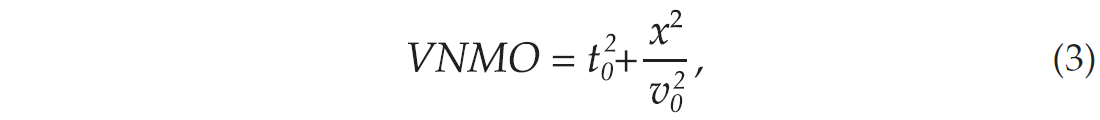
They view the anisotropic moveout equation as composed of three components, vertical normal moveout (VNMO), residual normal moveout (RNMO), and higher order moveout (HMO). Using their notations, equation (1) can be rewritten as,

where

and

Yang et al. (2002) proposed a procedure for the correction. Equation (3) can be used for a vertical velocity analysis if the traveltime can be corrected as if the wave propagates through an isotropic medium with velocity Vo. It involves three steps: (i) using short-offset data and conventional NMO equation to find Vnmo; (ii) using long-offset data to scan for Rh and Eq. (5) to correct the traveltime affected by an elliptic wavefront; (iii) rescanning long-offset data for Vnmo and using Eq. (4) to correct the traveltime affected by δ.

Banik et al (2002) used this approach and showed that the effect of anisotropy on seismic velocities could be as much as 8%, especially, in environments with thick shales. This can lead up to 2 ppg correction to predicted pore pressure (Banik et al 2002).

Post stack Inversion

The post-stack amplitude inversion concept is essentially based on 1-D inversion of seismic data. It visualizes the earth as a series of layers at each CMP location. Each layer is characterized by density, velocity and layer thickness. The earth model is discretized and sampled such that each layer has equal two-way time intervals. The procedure converts estimates of the reflection coefficients into an image of acoustic impedance with depth. Lavergne and Willm (1977) and Lindseth (1979) discuss the procedure in detail. Except for some modifications to take advantage of today’s computing environment, the basic approach remains unchanged. For normally incident pressure waves, the reflection coefficients for layer interfaces are related to the acoustic impedance by

where C_k is the reflection coefficients of the k^th interface and ρ_kv_k is the acoustic impedance of the kth layer. Then, the acoustic impedance for the next k+1^th layer is,

This operation is often called ‘trace integration’. It is, however, complicated by the fact that the field data lacks the low frequency trend (0-5 Hz, for example). Lindseth (1979) suggested using a velocity analysis approach to the high frequency impedance. This procedure is still used widely. Using a relationship between density and velocity, the acoustic impedance traces are converted to velocities. Thus, each seismic trace in the stacked data domain is converted into a pseudo-well velocity log trace. These velocities can be used for pressure prediction (Dutta and Ray, 1997). Kolb et al (1986) showed some excellent examples of non-uniqueness inherent in the method and showed very clearly that the low frequency trend in 1-D inversion is critically important.

Prestack Full Waveform Inversion

Velocity analysis tools discussed above provide velocities in the low-frequency regime. Although these velocities provide valuable information about pore pressure in order to define the seal integrity of a prospect, it may not be useful for drilling applications where mud programs and casing point locations require higher resolution. In these cases, prestack inversion of velocities from seismic amplitudes is very useful and especially suited for drilling applications. Further, prestack full waveform inversion, has the advantage of providing estimates of shear velocity in addition to a high resolution P-velocity (Mallick, 1999). The Genetic Algorithm (GA) inversion (Mallick, 1999) is an optimization algorithm used to find a suitable P- and S-velocity earth model by minimizing the misfit between observed angle gathers and synthetic ones. During the inversion process, an automatic NMO correction is performed first, yielding an initial RMS velocity. Next, interval velocities are derived from RMS velocities and a background density is determined as a function of depth from the interval velocity field. In addition to the moveout information, the GA inversion then uses the amplitude variation with offset (AVO) of the NMO-corrected prestack gathers to determine initial density and Poisson’s ratio values. Once the initial model is selected, GA generates random earth models within certain search bounds. It then uses standard GA search algorithms to find the optimum earth model that generates synthetic seismic data, which matches the input seismic data using exact wave equation. This exact modeling method can calculate all primary, multiple, and mode-converted reflections. Consequently, all interference or tuning effects due to thin layers and transmission effects due to velocity gradients can be accurately modeled in the inversion process. Since GA uses a statistical optimization process in searching for the elastic model, it also generates a measure of the uncertainties in the estimation of the elastic model.

Example Applications

Pore pressure imaging in 2D / 3D as well as predictions in 1D are useful for many purposes: regional seal mapping and seal integrity analysis for trends of hydrocarbon deposits and hydrocarbon migration pathway analysis, prospect high-grading and well planning that includes casing point design and mud program recommendations. The examples below are intended to highlight some of these applications.

Regional mapping of hard geopressure

A successful exploration program for hydrocarbon deposits involves three critical steps in the geophysical and geological processes: establishing the presence of reservoir, source rock and seal. In most of the accreting and subsiding Clastics basins of the world, the source rocks are usually buried very deep. The Gulf of Mexico’s tertiary basin is a good example of this. In these types of basins hydrocarbons are expelled at deeper depths, overcome capillary pressures and migrate upwards and laterally through fractures and faults. Creation of fractures and faults are directly related to sediment loading (growth faulting, for example), compaction and pressure buildup in low permeability sediments. Shale permeability measurements have indicated that at the depths typical of hydrocarbon reservoirs their values can be of the order of nano-darcies (Dutta 1987; Katsube 2002). Such low permeabilities create pressure traps and lead to seal development. In many cases, the pressure buildup is so rapid due to rapid burial rates, such as during the Pliocene time in the Gulf of Mexico, that seals often breach. This causes the trapped fluids (brine, hydrocarbon) to escape and pressures begin to drop, causing closures of the fractures. Events such as these may even be episodic during geologic times (e.g. Walder, 1984). Thus, one needs to know the pressure state at which such an incident (seal failure) may happen. Although there is no agreement as to how high the pore pressures become before they fail, it has been our experience through many well log analyses that this usually happens when the effective stress in the seal becomes low, 750 Psi to 1000 Psi, for example.

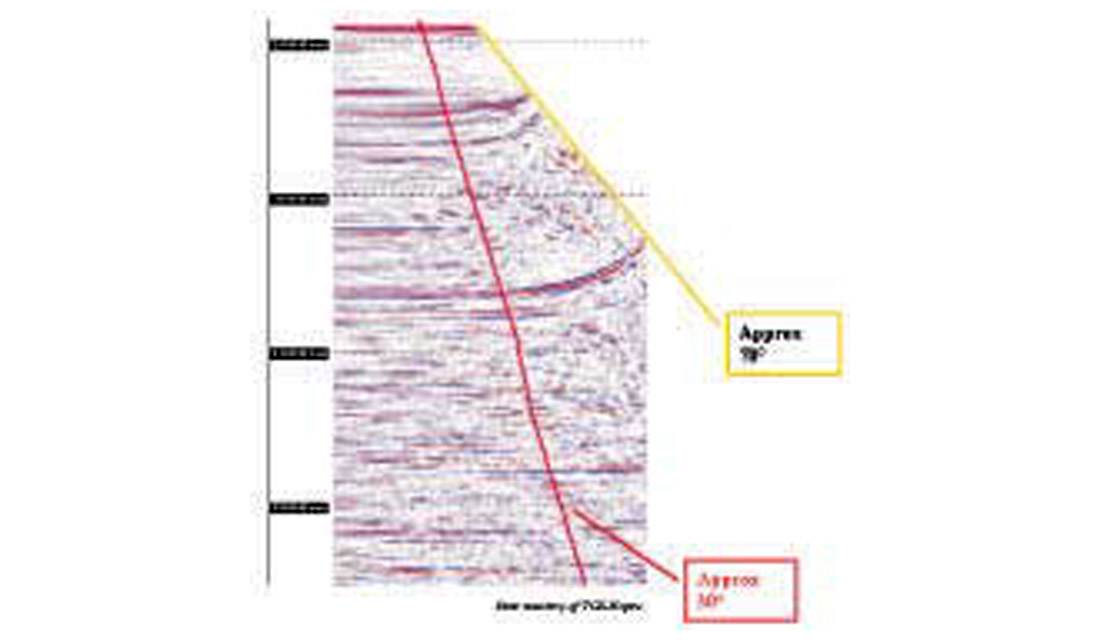
For 3-D applications (for regional pressure work) velocities come from either a 3-D velocity survey or a grid of closely spaced 2-D seismic lines. Typically, such analyses proceed in several stages. The First phase essentially consists of a calibration phase of interval velocities derived from the conventional stacking velocities using available well controls. This step requires access to a 3-D gridding software where velocity conditioning, including lateral and temporal smoothing and interpolation, is carried out. Salt masking and other quality control steps are also applied at this step. A critical step is the anisotropy correction as discussed earlier. This requires an access to seismic data with as large a cable as possible. In Fig. 7 we show the effect of data acquired with a large cable on velocity moveout; clearly, a large offset data will yield a better velocity function than those acquired with a cable that yields a smaller offset (30 degrees, for example). The data is from deep water NW shelf of Australia (Canning Basin) and acquired with a 6km cable length.

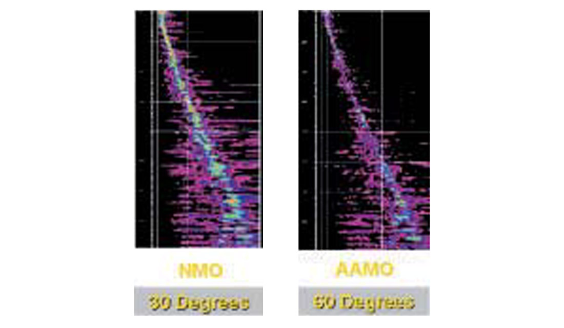
Figure 8 shows the effect of the anisotropy correction on a single gather; the plot on the left is the velocity spectra of a single gather with the conventional processing, and the one on the right is the same data after correcting for the anisotropy effect. We note the improved quality of the spectra allowing for a velocity analysis with more reliability and confidence. For pore pressure analysis, such improvements in velocities can easily lead to reducing the pressure uncertainty by as much as a 1 ppg at the typical target depths.

The output of the above process is a velocity cube in 3-D, which is then loaded on a seismic workstation and visualized using any visualization software. The next phase of the process deals with transforming the 3-D velocity cube to a cube of 3-D effective stress or pressure. The transform is based on rock models such as those discussed in Mukerji et al (2002) or Dutta (2002). The subsequent phase consists of depth conversion using the velocity data, so that the pressure maps can be displayed as a function of depth, and not two way time. The last phase of the process consists of taking slices of the pressure cube along major horizons and projecting them in map view. This allows us to get a better understanding of the relationship between pore pressure and the occurrence of the major sand and shale units.

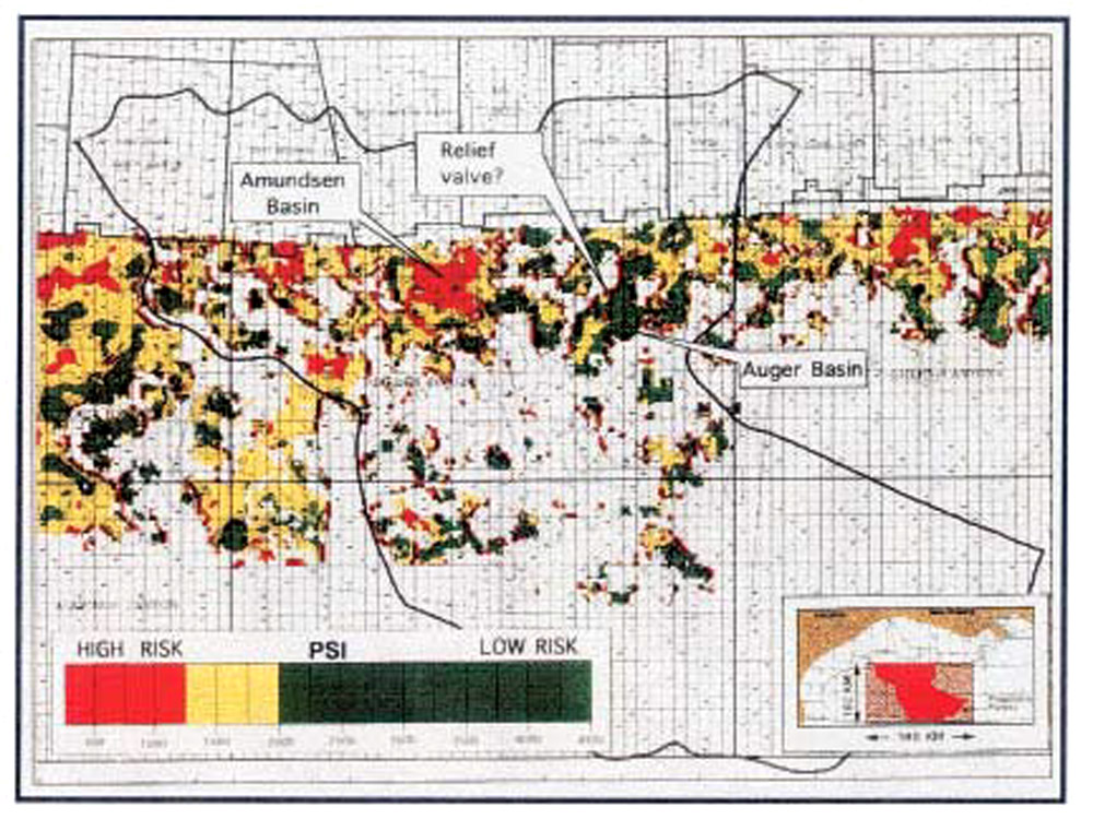
Figure 9 shows an application of this procedure, taken from Dutta (1997) from the deepwater, Gulf of Mexico. The area of study is shown in the inset. Here a 3-D model of effective stress has been developed over a prospective play fairway. The model covers an area of 140x102 km, with water depth greater than 330 m. Figure 9 is a map of the effective stress, in psi, and projected at a prospective horizon over many blocks. The color codes in this figure represent the risk associated with hydraulic seal failure; red denotes high probability of seal failure. This sort of maps has helped the explorationists to high-grade the areas of low top seal risk, and downgrade risky areas.

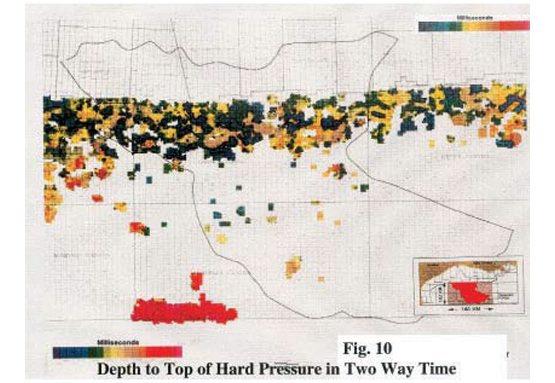
Figure 10 is a map of top of hard pressure in the same fairway (deep water Gulf of Mexico) as a function of two way time. Here the top of hard pressure has been defined as that depth (or time) where the effective stress reaches a threshold value of 1000 psi. Analysis such as the ones shown here in 3-D, should always use the gridded velocities which are no more than 0.25 km apart. Otherwise, the interpolation process in 3D rendering may create a geology that is neither present nor realistic.

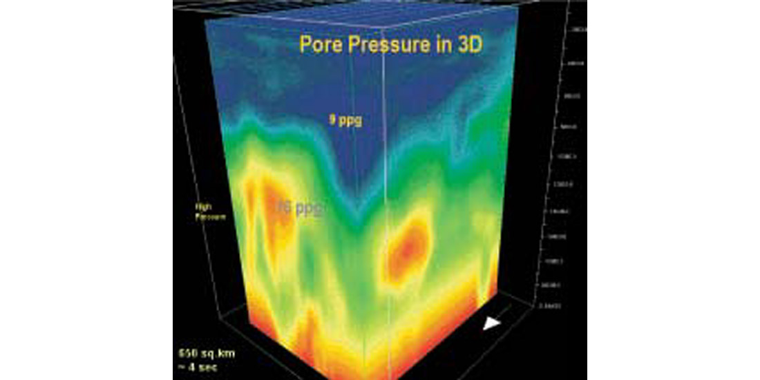
Figure 11 is an example of the SCVA/ AVMB procedure on a 3D data set, used for an improved prospect definition in a region that is about 650 square miles. The velocity analysis employed here used semblance data at every CMP. We see significant clarity of the pressure image in 3D, and the high-pressure pockets (greater than 16 ppg mud weight equivalent) are clearly visible (red).

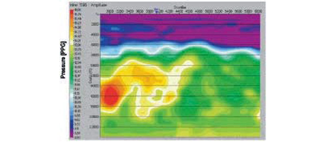
Figure 12 shows a cross-section of the same 3D cube in 2D along the prospect. It clearly shows high-pressure pockets and the effect of differential compaction due to fluid transport. Clearly, the prospects within the high-pressure trap may not be as desirable as those outside. The pressures might be too high inside the region denoted by red and seal might have been mitigated in that area in the geologic past.

Prospect high grading by pore pressure imaging

Geopressure can cause drilling problems. However, they also provide a trap for hydrocarbons. Timko and Fertl (1972) drew our attention to a distinct relationship between hydrocarbon accumulation and geopressure and its economic significance. These authors showed that in the majority of cases, the economic hydrocarbon deposits in the Gulf of Mexico occur in low to moderate pressure regimes (the fluid pressure gradient regime between 0.5 psi / ft to 0.8 psi / ft. Explorers for oil and gas often look for such traps using geological models and seismic data in 2D and 3D. Thus, one can high-grade exploration portfolio using pore pressure as a criterion.

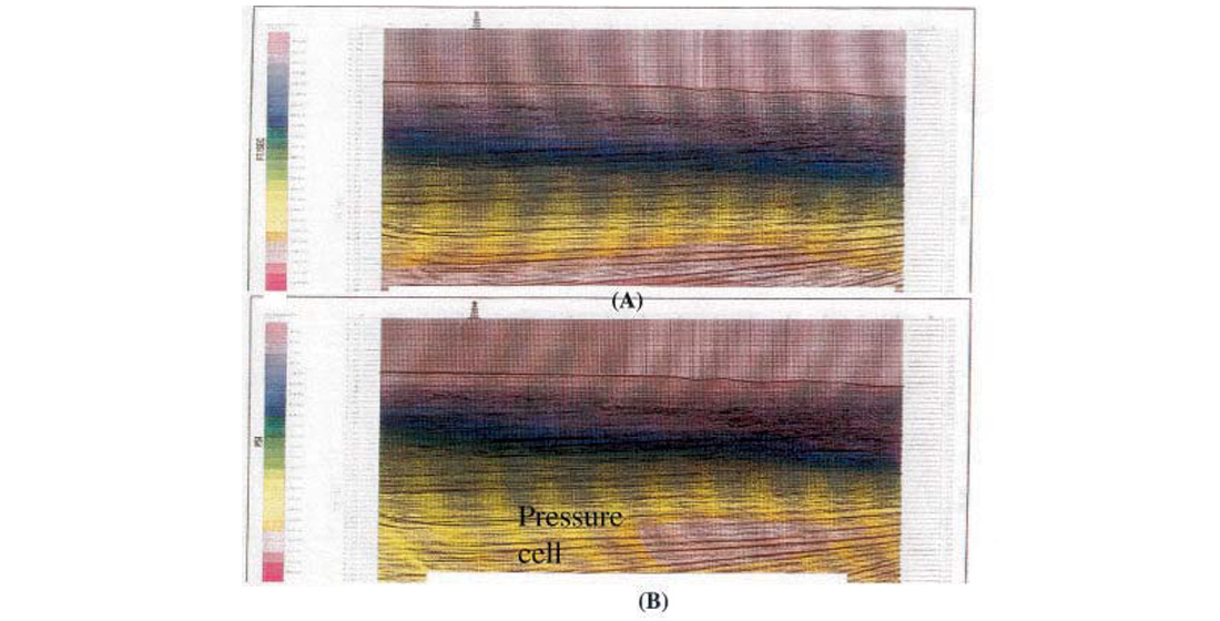
Another example from the deepwater Gulf of Mexico is shown in Fig. 13. The top half of this figure shows the seismic interval velocities in color in ft / sec together with stacked traces. We note the general conformity of the structure with the interval velocity field derived from the stacking velocity data. The predicted 2-D cross-section of the effective stress, in psi, is shown in the bottom half of Fig. 13 as a function of two-way time and the CDP number. The color scale of this figure ranges from 470 to 4150 psi. A gradual increase of effective stress (meaning a decrease in fluid pressure) is apparent from left to right (away from the well). This suggests relatively more compaction (and consequent expulsion of water) as one moves away from well and moves updip to the right. Thus, an increase in the effective stress up-dip and away from the well location suggests an active migration pathway of fluids.

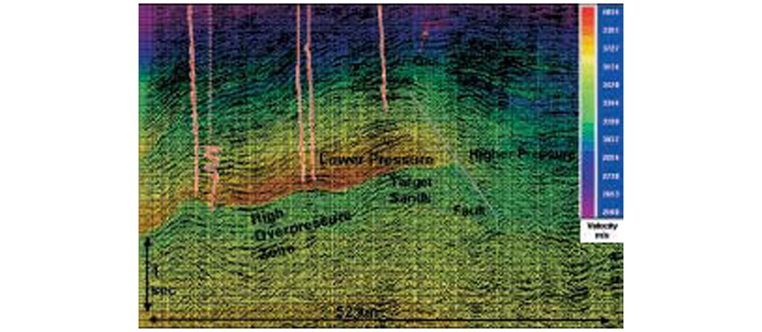
An example of the use of tomography and prestack depth migration is shown in Figure 14. This figure shows a clear transition from low pressure to high pressure in a dramatic fashion. We also note the pressure across the major fault is much higher (to the right). Thus it appears that the fault is clearly a ‘sealing fault’. Quite often such pressure transitions are very rapid and require an extra string of casing to control the high formation pressure during drilling related transients.

Pore pressure analysis and applications at well bore scale for drilling

The examples that we presented so far deal with low frequency analysis of pore pressure. Velocities are obtained from either semblance analysis of stacking velocity data or from tomography and prestack depth migration. However, for drilling applications one requires higher frequency predictions. Such predictions require using velocity as well as the amplitude data. First, the best low frequency model is established at the well location. These velocities are then calibrated with the analogue well data, if available. Both sonic and VSP logs are very useful for this purpose. Next, high frequencies are superimposed on the low frequency data by obtaining seismic velocities from seismic inversion of amplitudes. In the early part of this paper, we suggested two approaches for this; post stack and pre-stack inversion of amplitudes at the well location. Below we present some examples.

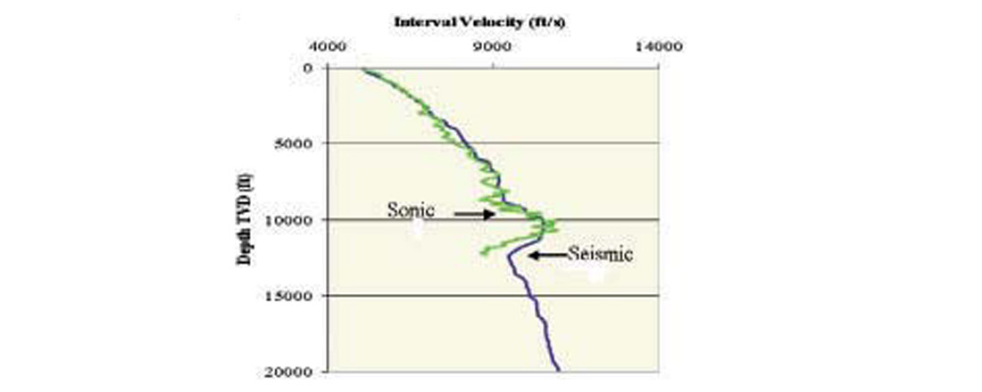
Figure 15 shows an example of the low frequency model that is improved by inversion at a well location. The low frequency model is from the velocity analysis of semblance data using the horizon consistent velocity analysis. The high frequency curve superimposed on this is the sonic well log from the analogue well. It suggests that the seismic velocity data yielded the trend of velocity remarkably well. It is highly desirable and recommended that such calibrations be performed prior to any application of seismic for pore pressure analysis for well planning. Only then adding high frequencies will make sense. Otherwise, inversion will result in just noise!

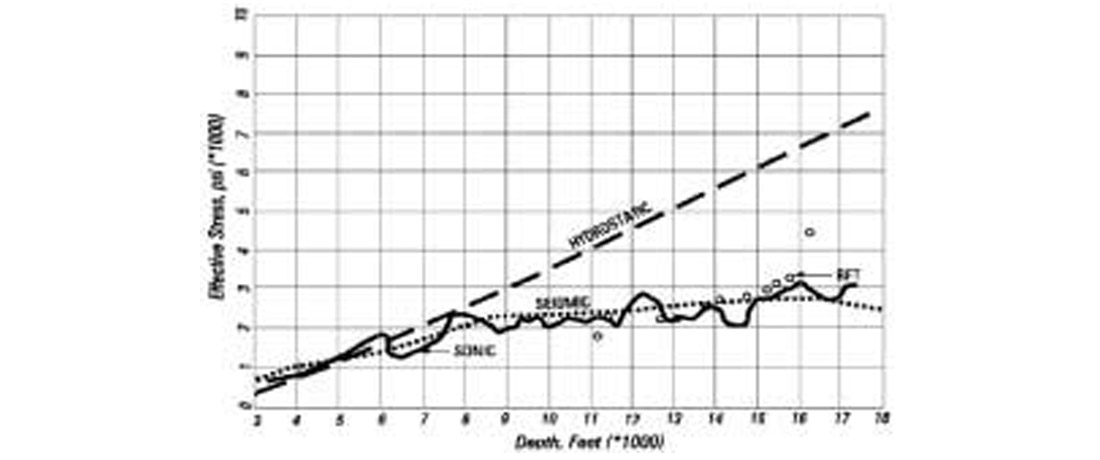
Figure 16 shows a comparison of the band passed calibrated sonic log and seismic interval velocity at the well location: the two velocities are in good agreement showing a general goodness of the velocity analysis of the reflection seismic data. The predicted effective stresses from both seismic and sonic are shown in Fig. 17. The line marked “hydrostatic” shows the expected effective stress variation, had the fluid pressure been in hydrostatic equilibrium. The Geopressure in this well began at approximately 6 kft below the seismic datum where the predicted effective stresses depart from the hydrostatic line.

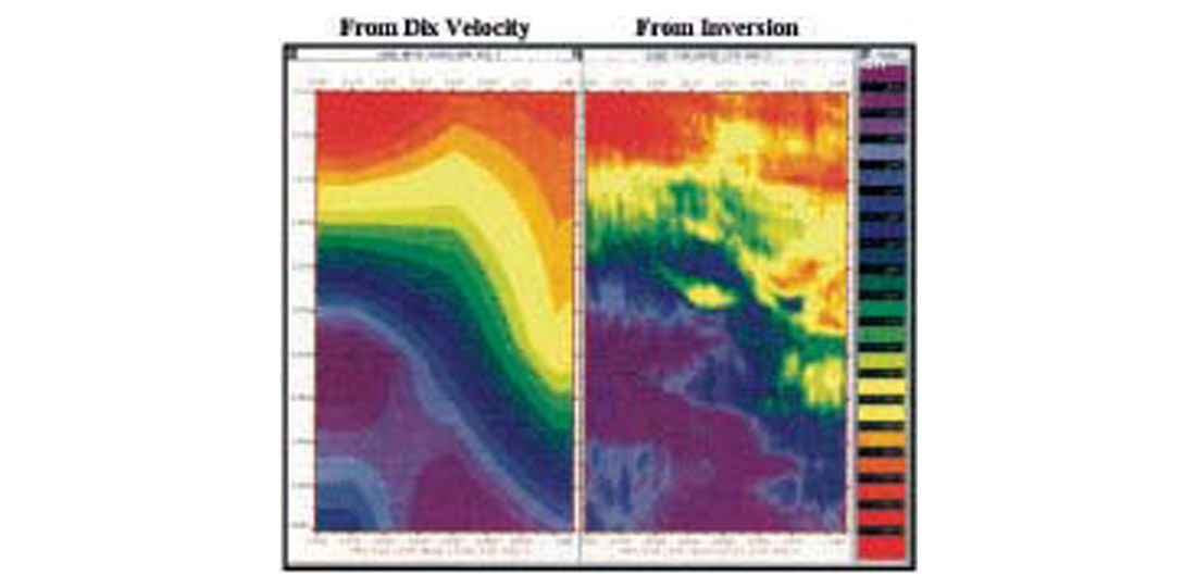
Figure 18 shows an example of post stack inversion from the deepwater Gulf of Mexico. This figure is a plot of the effective stress, in psi, versus tow-way time for every CMP location. The data are from a field in the deepwater, Gulf of Mexico (Dutta and Ray, 1997). The left side of Fig. 18 uses the Dix model, while the right side figure uses the high-resolution velocity model from post stack impedance inversion. The improvement in the spatial resolution of estimated effective stress in the latter model is obvious; the seal distribution around the bright spot is clearly visible in the right side of the figure at about 3400 msec. Further, an additional reservoir at about 3340 milliseconds is also visible.

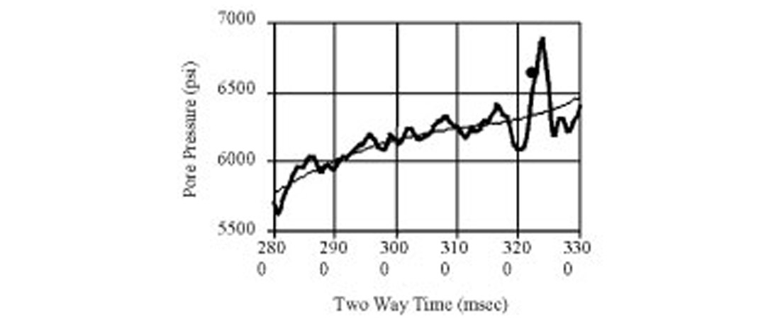
Figure 19 shows a plot of the high-resolution pore pressure, in psi, versus two-way time at the well location (full line) and a comparison with RFT data (black dot) taken within the top reservoir. The thin line in this figure shows pressure estimate from the Dix model. We note that the high-resolution velocity model predicts the pressure reversal at the reservoir level. The Dix model does not yield such detail; it just provides a low frequency pressure trend.

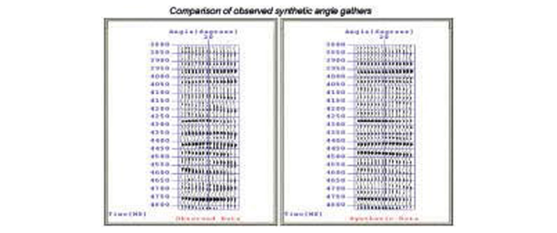
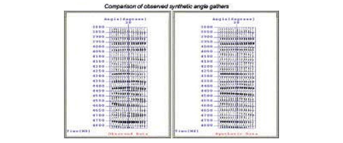
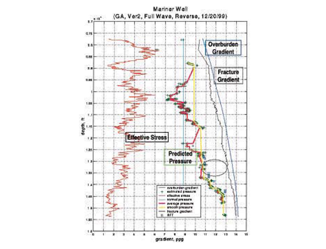
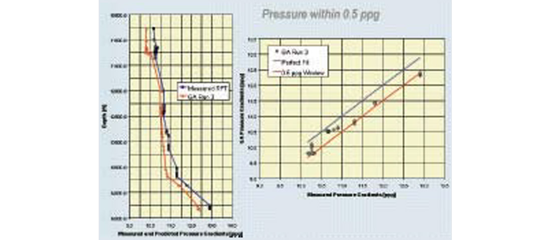
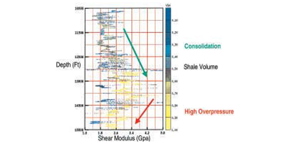
Example applications of prestack and full waveform inversion are shown in Figs. 20-24. Figure 20 shows the single CMP gather at a well location from a deep water environment in the Gulf of Mexico (water depth ~ 5200 ft) and that obtained from the full wave form pre stack (GA) inversion prior to drilling. The agreement is good. Figure 21 compares predicted velocity logs (P and S) to those obtained from the post drilling. A comparison of the predicted pressure profile with those from drilling data (Figs. 22 - 23) indicates that the predicted pressures are in good agreement with the measured values to within 0.5 ppg. Figure 24 shows a comparison of the predicted shear modulus, again from the prestack full waveform inversion, with those from recorded shear sonic data. It suggests that Poisson’s ratio versus depth predicted using prestack inversion could be a powerful tool for estimating this important attribute prior to drilling- perhaps more meaningful than those obtained using AVO (small offset, linearized inversion). We note that prior to the overpressured ramp in this well, the shear modulus increases with depth due to increased compaction, as expected. However, when the pressure ramping takes place, indicated by a 15% increase of pore pressure, the shear modulus decreases by almost 25%. This is remarkable and suggests that both shear-wave data and very large offset P-wave data may be very good indicators of high pore pressure.

Applications to Shallow Water Flow (SWF) formations for hazard identification in deep water

Shallow water flows (SWF) are frequently experienced in deepwater areas when drilling into poorly consolidated geopressured sands (Fig. 25). These sands, when flowing, can cause extensive damage to a bore hole and the well site. For instance, over $200 million was lost to date remedying and preventing shallow water flow problems in the Gulf of Mexico alone. In an extreme case the problems led to loss of several wells that were pre-drilled through the over-pressured sands. As the result the development site had to be relocated. According to a report from Fugro Geoservices, approximately 70% of all deepwater wells in the Gulf of Mexico have encountered SWF. Lately this problem has also been a concern to drillers in many other deepwater Clastics basins of the world, such as Mediterranean, Angola, Nigeria and Brazil.

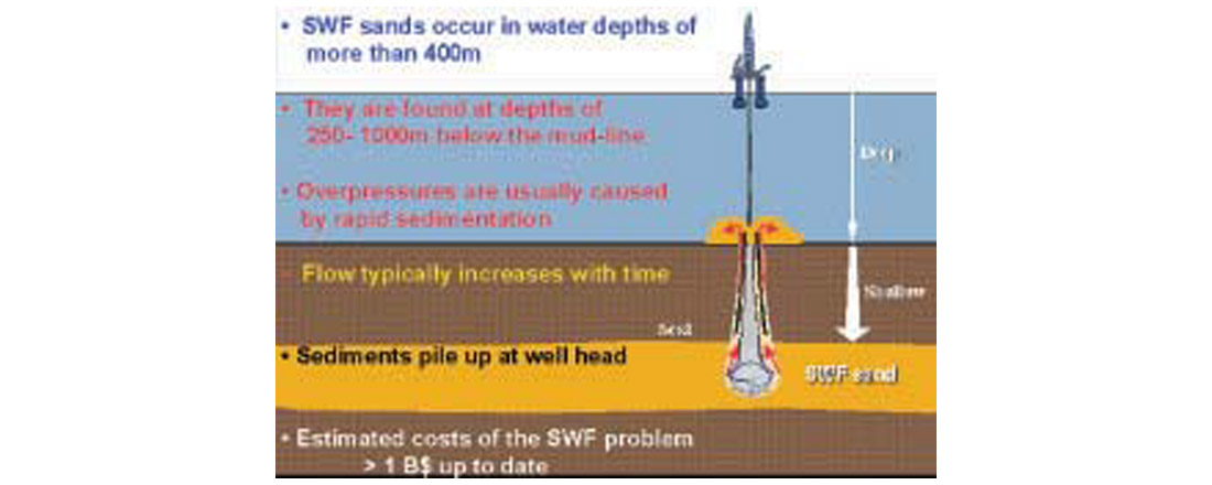
Shallow waterflow sands are known to occur in water depths of 450 m or more and typically between 300 m and 600 m below the mud line. They are found in areas with high sedimentation rate all over the world. The shallow sands, when sealed from the rapidly building overburden, remain extremely porous under increasing overpressure, rendering them highly unstable. Reliable detection of potentially hazardous shallow water flow situations is a key to controlling the problem and for managing the associated costs. Seismic techniques in conjunction with geologic analysis of stratigraphic sequences related to SWF zones are useful in detection of these hazards prior to drilling. The rock properties of these sediments have been discussed in Mukerji et al (2002). A key parameter is the Vp / Vs ratio, which is very high for these sediments.

Seismic detection options for SWF formations

Seismic data has long been recognized as a key to SWF detection prior to drilling. An elegant approach suggested by Huffman and Castagna (2001), using multi-component data, is the preferred approach, although it is very costly in terms of the current state of the technology. Further, there are hardware limitations that prevents for that technology to be extended to ultra-deepwater (water depth in excess of 5000’). AVO approaches are also limited in usefulness; these do not provide reliable estimates of Vp/Vs ratios, since various physical phenomena such as reflections from hidden layers, multiples, mode conversions and various reflection and transmission effects are totally neglected. These effects become important at large offsets (greater than, say, 25⁰) .

In the applications discussed below we suggest an approach based on prestack and full waveform inversion of seismic data that allows us to quantify the rock properties of SWF formations using the entire offset range of conventional 3D seismic data. Further, the methodology uses the geologic model building aimed at understanding the stratigraphic and structural control on SWF formations. DeKok et al (2001) discussed some aspects of this approach earlier. The application to SWF identification involves the following steps. These are: reprocessing seismic 3D data at 2ms samples with special care for S/N enhancements and amplitude preservation, stratigraphic analysis of the data to locate possible horizons that may contain SWF sands with possible existence of local seals, attribute analysis (AVO for example) of the 3D cube for verifying the seismic signature of SWF formations, prestack full wave form inversion of the gathers to obtain high frequency profiles of Vp, Vs and density, and finally, using a rock model to estimate pore, fracture and overburden pressures.

Examples from real data sets

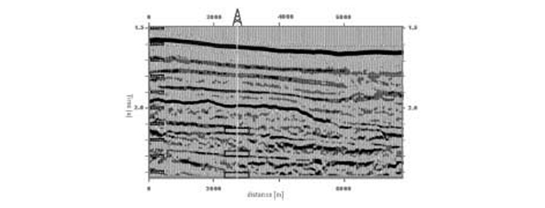
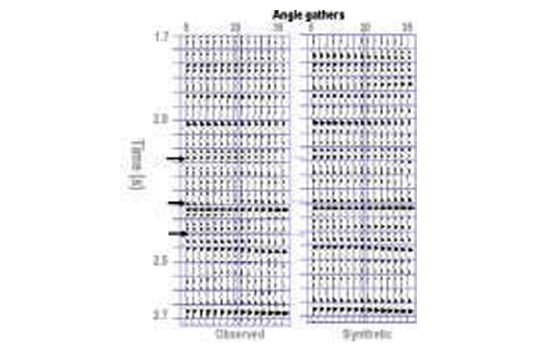
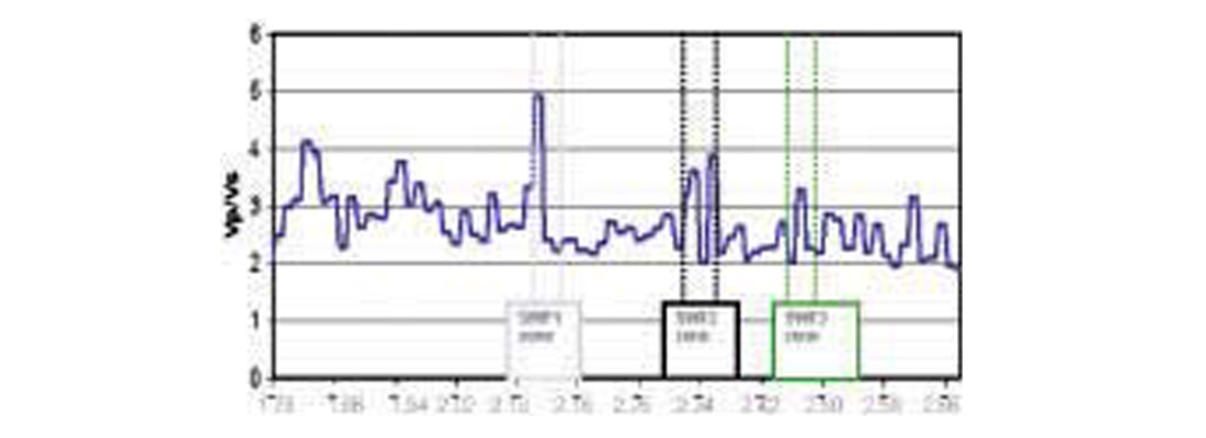
For tests on real data, we selected a 3D seismic data volume from the Gulf of Mexico (Mississippi Canyon area, offshore Louisiana). In this area, the SWF conditions are known to occur. The seismic data was reprocessed at 2ms sampling interval for high-resolution trace inversion. The key acquisition parameters are: source at 7m depth, streamer at 10m depth, 80m shot interval, 4800m streamer length and 30 fold multiplicity. The data was processed in a 2D sense because the binned data exhibited abrupt amplitude changes versus offset not related to geology but rather to contributions from different source to streamer combinations. The geometry related offset changes manifested themselves as the amplitude and reflection time discontinuities. A 2D stacked section, reprocessed at 2 ms is shown in Figure 26. The well is indicated with markers at the three SWF levels. As input to prestack inversion, the data were corrected for divergence, but not for absorption, and zero-phased without further deconvolution. In spite of a strong P-wave contrast, on a stacked section the reflection strength of the SWF sands is weak, often making them less visible than other sands. This is due to the Type II AVO behavior, leading to a polarity reversal around 30 degrees in this particular case. The results of prestack inversion are shown in Fig. 27; the figure on the left shows the angle gather at the well location, and the one on the right shows the results from GA inversion. Figure 28 shows the synthetic Vp/Vs log obtained from the prestack inversion. Note the high values of this attribute at the SWF locations.

It verifies the discriminating ability of the Vp/Vs ratio. Anomalous high values appear at the levels where SWF layers were experienced during drilling.

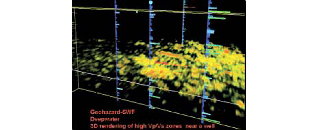
The procedure described above has been carried out in 3D also using the 3D hybrid inversion approach developed by Mallick (1997) and applied to a SWF problem by Mallick and Dutta (2002). In this approach, GA inversion is performed at several locations in a 3D data volume after carrying out the stratigraphic analysis. The GA inversion is designed to obtain both low and high frequency velocity variations through the simultaneous modeling of move-out and elastic reflection amplitudes. The inter-well space is then filled by AVO inversion using the trends of Vp, Vs and density obtained from the GA inversion. An example from the deepwater Mediterranean is given in Figures 29-30. Figure 29 shows a portion of a 3D seismic data volume that indicates the possible existence of SWF formations based solely on the stratigraphic analysis. Figure 30 shows a 3D analysis of the Vp/Vs ratios using the 3D hybrid inversion procedure. The color indicates numerical values of Vp/Vs ratios – it ranges from 2 to 25. The high values are possibly associated with the SWF formations.

Conclusions

This work suggests that formation pore pressure could be predicted from seismic data provided care is taken to condition the velocities to appropriate rock models and to ensure that the rock velocities are extracted from the seismic velocities. The analysis and examples show that as large an offset as possible should be used for pore pressure imaging. Further, a fit-for-purpose velocity tool should be used. Thus, tomography and prestack depth migration should be used when significant imaging problems and ray-path bending effects are encountered. In most cases, prestack time migration may suffice, provided the geology dictates a meaningful application.

Prestack full waveform inversion is found to be a powerful tool. It yields pore pressure versus depth profiles with more vertical resolution than feasible from the conventional velocity analysis. The resulting Poisson’s ratios can be used for obtaining fracture gradients as well as lithology prediction. High frequency pressure variations from inversion make it an attractive technology for drilling applications

Acknowledgements

We thank WesternGeco for the permission to publish this paper, and we acknowledge the support from sponsors of the Stanford Rock Physics project.