SAGD Well Planning Using Stochastic Seismic Inversion

Abstract

The complexity of heavy oil geology in SAGD (Steam Assisted Gravity Drainage) projects, especially in the presence of thin shale barriers that are beyond the resolution of traditional deterministic seismic inversion, makes the integration of seismic data with well data challenging. Stochastic inversion represents an improvement over deterministic inversion in that it can provide finer reservoir detail through the generation of a large number of possible high-frequency models that can be used for post-inversion analysis of facies and connectivity. As part of the process, probability estimates of continuous reservoir, continuous shale and producible bitumen are created.

This paper explains these techniques and shows how they were used for SAGD well planning. The results of the inversion were post-processed to generate bitumen and shale probability cubes and to highlight zones of thick continuous bitumen. A number of maps and 3D surfaces were then generated, allowing the positioning of a set of horizontal wells taking into account various probabilistic quality indicators. Finally, an estimation of the volume of bitumen that could be drained from these wells was computed and used to rank all stochastic realizations in order to identify P10, P50, P90 cases.

Introduction

There is a growing demand in seismic reservoir characterization studies to quantify uncertainties in the results of techniques such as inversion and to obtain realistic geological models.

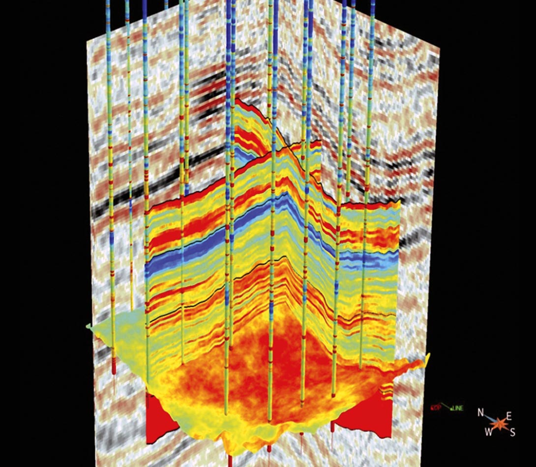
Stochastic seismic inversion can address this demand by generating a suite of possible elastic rock property models (typically hundreds), all honouring the seismic, well, and geostatistical inputs, with vertical resolution similar to that of the well logs (Figure 1).

After an introduction to the stochastic concept, a SAGD project will be used as a case study to illustrate why this type of characterization should be considered.

The spatial variability of the geology in heavy oil plays combined with the close spacing of wells make these fields ideal case studies for the statistically intensive technique of stochastic inversion.

Introduction to stochastic inversion

Stochastic modelling has been used in geology for more than 30 years, to produce geologically plausible models honouring all the known sparse information, such as well logs, trend curves and sedimentary settings, as well as to study the uncertainty associated with these models (Chiles and Delfiner, 1999). In recent years, it has been used in geophysics as well, particularly for seismic inversion (Gunning, 2004). There are different families of stochastic inversion algorithms, from simple acceptation/ rejection schemes (Haas and Dubrule, 1994) to more complex Bayesian formulation.

Although the actual equations can be quite complex, the principle is simple, and an example of a submarine cable may be useful to illustrate why the stochastic concept is interesting to geoscientists. In this example (Figure 2, upper left), the objective is to estimate the length of cable required to cross the sea floor using only sparse depth sampling, before laying down the cable. It would be unfortunate to run out of cable before reaching the coast while it would be uneconomic to load excess cable that was surplus to requirements. What length of cable must be loaded on the ship for installation?

Different interpolation techniques such as straight interpolation or kriging can be considered but they typically underestimate the true length (Figure 2, centre left) and are, therefore, biased. To overcome this problem, stochastic simulations can be used to create multiple scenarios, each of which honors the sparse sampling but varies between the sampled points, with a local variability constrained by a variogram. It is impossible to know if any single realization matches the reality, or which one is closer, but an analysis of the multiple scenarios can be used for uncertainty measurements by creating a range or histogram of possible lengths within which lies the correct answer (Figure 2, bottom left).

From this example, an analogy can be made with seismic data which usually has good lateral resolution but which has a vertical resolution limited by the seismic frequency bandwidth. The stochastic technique can be transferred from the horizontal scenario of determining the detail of the sea floor, to the vertical scenario of determining the detail of a P-impedance well log (Figure 2, right).

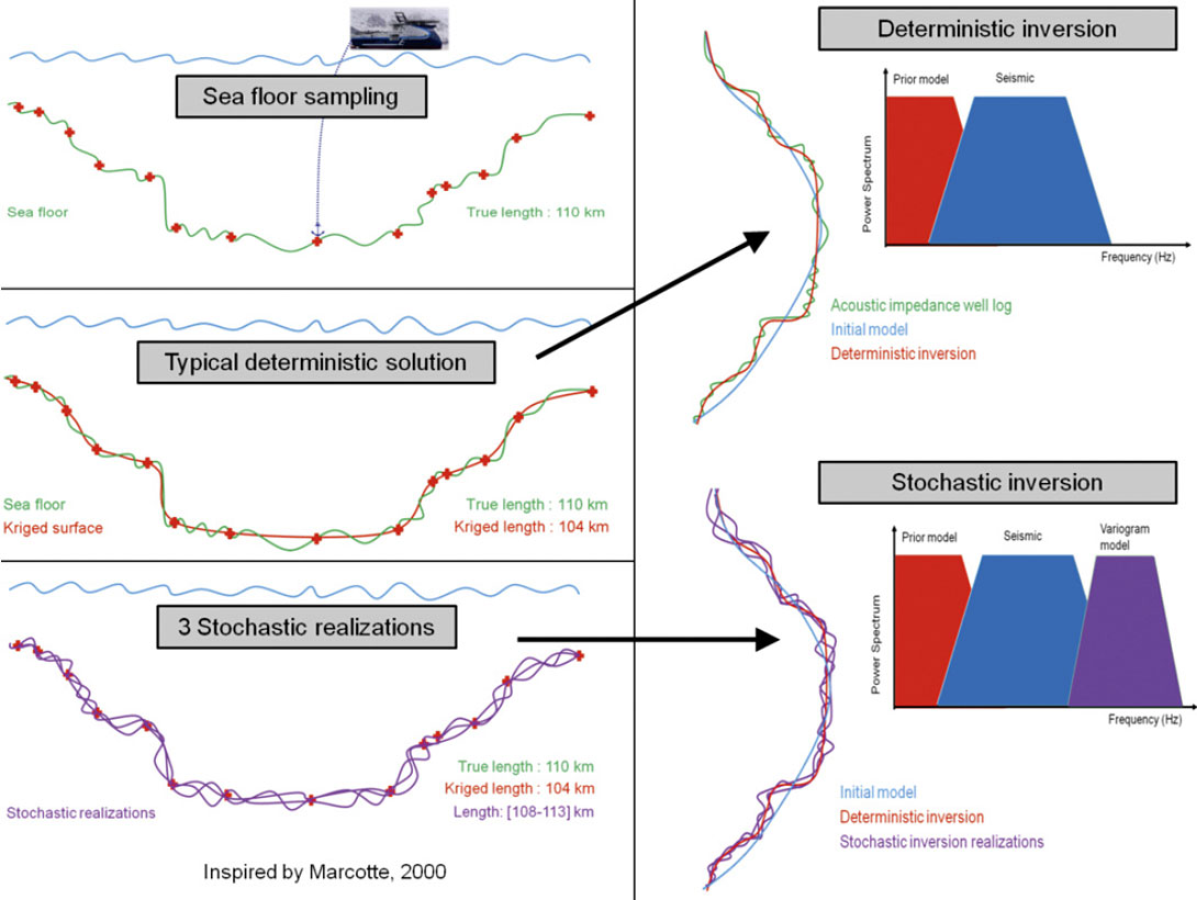
As in most seismic inversion techniques, an initial model is required to provide the low frequencies that are not typically present in the seismic. With a deterministic inversion alone, details will be smoothed and heterogeneities, such as thin shale barriers, will be underestimated. However, each realization from a stochastic inversion will contain a range of frequencies similar to those in the well logs (i.e. higher than the seismic). As in the marine cable example, no one realization can be regarded as the single solution and analysis of the stochastic results is required in order to translate the uncertainties from the elastic attributes into the geological/engineering properties needed for SAGD well planning. This post-inversion analysis will be discussed further in a later section.

In Figure 2, only three realizations are shown but stochastic inversion usually involves hundreds of realizations in order to guarantee that enough scenarios are sampled. The precise number is controlled by the variogram and the number of layers (vertical resolution) in the initial model. The best way to calculate the correct number of realizations is to examine the histogram of the final product (for example the length of the marine cable) and check when the mean, the median and the standard deviation of the histogram become stable, i.e. when adding more realizations will not change these values.

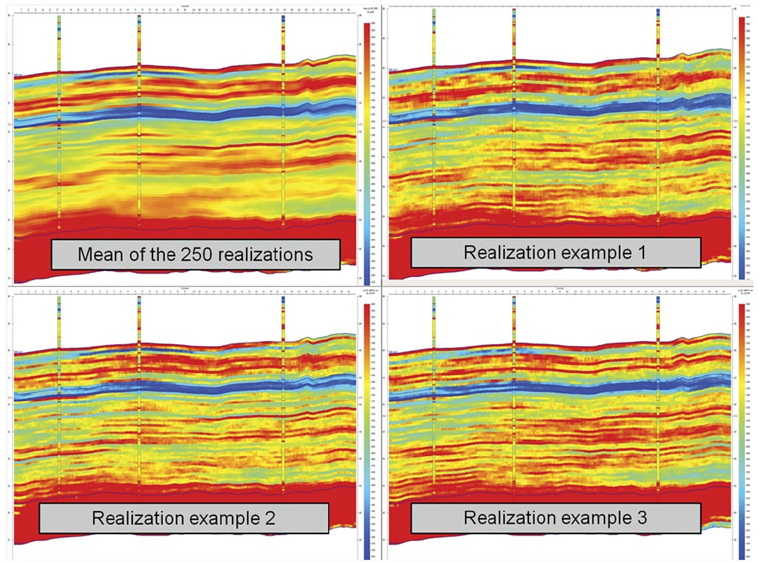
The stochastic process mostly affects the high frequencies, averaging all realizations results in keeping only the frequency content of the seismic. Consequently, the mean of all the realizations is very similar to the result of a deterministic inversion (Figure 4 shows the smooth character of the mean).

Variograms play an important role in this stochastic process. Although they will not be discussed in detail in this article, it is interesting to note that for stochastic inversion they will only constrain the high frequencies. The vertical variogram is usually easy to derive from well logs whereas the horizontal variogram tends to be defined more empirically and can be derived from secondary information such as the seismic when well control is sparse.

A case study using stochastic inversion

The methodology was tested on 1.25 sq miles of seismic data acquired over a heavy oil field in Alberta which contained 16 vertical delineation wells (Figure 1). The target interval was approximately 40m thick and contained bitumen sand, gas sand, IHS (Inclined Heterolithic Strata), shale layers, and calcite streaks. The sands are inter-bedded to a varying degree with muds which can be localized or spread over large areas. The seismic data comprised four angle stacks ranging from 6 to 28 degrees with frequencies up to 200 Hz. Statistical wavelets were extracted from the seismic.

The stochastic seismic elastic (pre-stack) inversion was performed using a Bayesian framework based on a linearized AVA model (Buland and Omre, 2003, Escobar et al., 2006) to calculate a joint posterior distribution for P- and SImpedances, constrained by seismic amplitudes measured on the four discrete input angle stacks. This posterior distribution was sampled sequentially and repeatedly to generate 250 alternative high-frequency 3D realizations of the elastic properties. The stochastic inversion was performed in a finescale stratigraphic grid defined in the time domain, with horizontal sampling fixed by the seismic bin size and vertical columns of cells with variable thickness, typically much finer (around 1ms) than the seismic resolution.

The inversion was directly constrained by the seismic data and also by the wells, allowing for better control of the higher frequencies where they are known (i.e. at the wells). Moreover, lateral and vertical variability was constrained through vertical and horizontal variograms extracted from the well data (Figure 3).

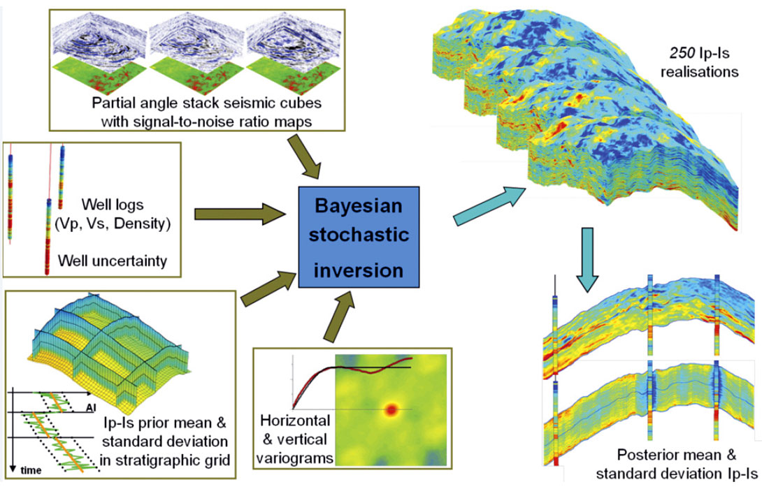
Figure 4 compares different outputs of the stochastic inversion: the P-impedance of the mean of all the realizations and three of the 250 realizations randomly chosen as examples of the variations in the detail.

These detailed models of elastic properties were then transformed into properties related to the geology and engineering problems of this case study using post inversion analysis.

Objectives of post-inversion analysis

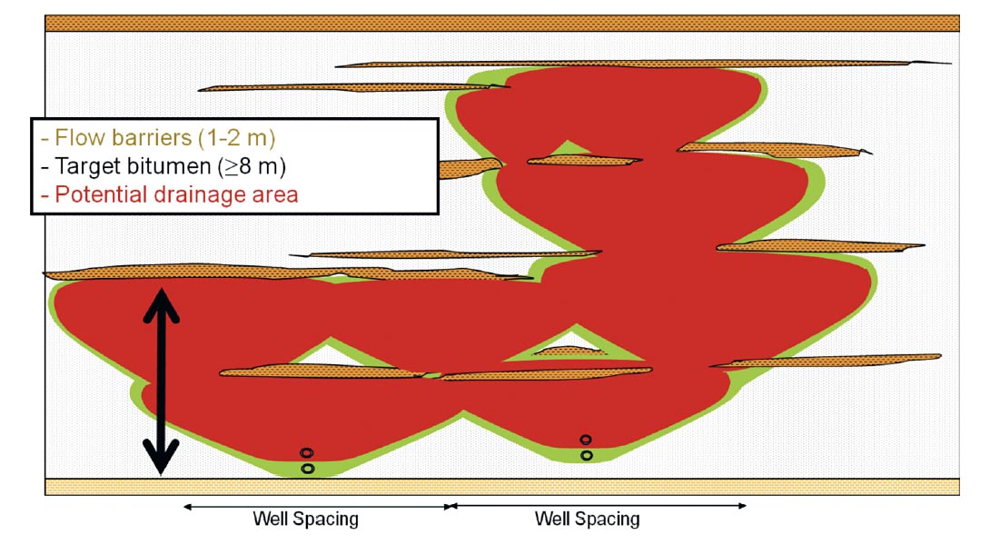
In a SAGD project, it is very important to define thin shale barriers that may impede steam chamber growth, to locate sweet spots of thick bitumen within which well pairs are to be drilled and to assess the vertical connectivity above well pairs (Figure 5).

The sequence, applied to all realizations, in this case study was:

1. Predict shale/sand facies from well impedance cross-plots.
2. Scan these facies volumes for continuous shale layers which could act as barriers as well as for thick and continuous target bitumen sands.
3. Map these scanned volumes for thickness and position (base and top) of target bitumen zones.
4. Use these maps to position potential well pairs.
5. Assess vertical connectivity (i.e. volume that can be drained) above these wells.

Facies classification

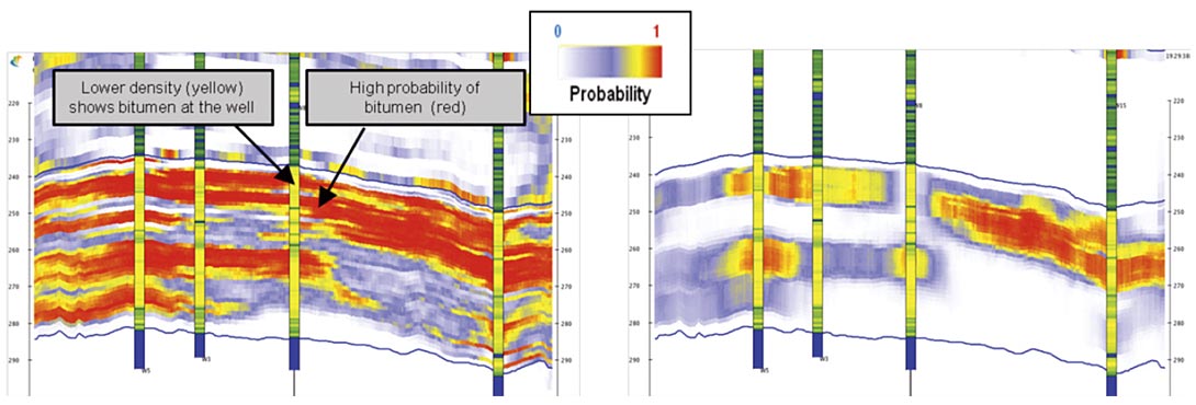
A standard way to exploit stochastic inversion results is to transform impedance realizations into facies (Moyen and Doyen, 2009). Analysis of 16 well logs within the study area, identified three target facies according to their lithology and fluid content: bitumen saturated clean sands, gas-filled clean sands and shales. Crossplots of P-Impedance versus S-Impedance for each well-derived facies, showed a good match to crossplots of the inversion-derived P-Impedance versus S-Impedance volumes, confirming that good facies discrimination was achieved. These zones were then applied to each of the realizations to produce 250 facies realizations. By counting in each cell and each realization, whether or not a facies is present, a facies probability cube can be computed, as shown in Figure 6 (left) and the uncertainty in seismic lithology prediction from the stochastic inversion can be estimated. (i.e. if 200 out of 250 realizations classify a cell as sand, there is an 80% probability of sand).

While determination of the facies is useful, for SAGD it is also necessary to go further and identify the lateral extent of shale layers which may be a barrier to steam flow; and to identify the vertical extent of bitumen.

Target bitumen and shale barrier detection

For optimum SAGD production, it is necessary to identify target bitumen zones that are suitable for pad placement, i.e. thick continuous bitumen sands (Garner et al., 2005). These sands are identified on each realization, using simple geometric criteria such as the minimum lateral extent of shales that could be considered a barrier, or the minimum thickness of clean sands required (8-10 m in this case). The realizations can then be combined to produce a probability cube of target bitumen (Figure 6, right).

Mapping

Mapping of the available attributes facilitates interpretation. Several statistical indicators can be computed:

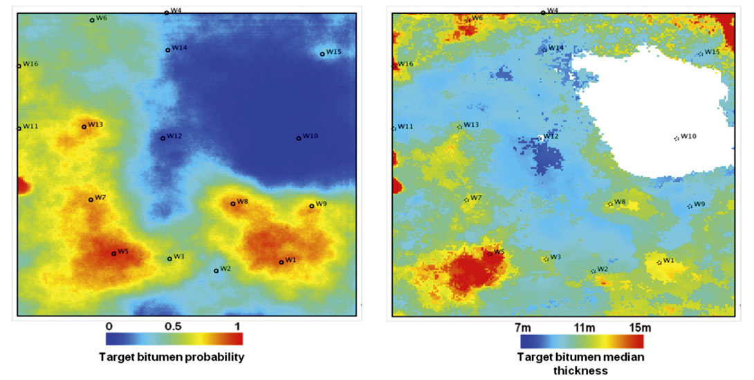
A map showing, the probability of target bitumen in each bin (Figure 7, left).

• Three maps (P10, P50, P90) representing pessimistic, median and optimistic scenarios of the depth of the base of the target bitumen zones (Figure 8, left).
• Three maps (P10, P50, P90) of thickness of the target bitumen zones. The median case (P50) is shown on Figure 7, right.
• Three maps (P10, P50, P90) of the thickness of the first shale layer above the target bitumen zones.
• It is important to note that these maps are statistical indicators computed from all the stochastic realizations. They do not correspond to one single realization.

SAGD Well Planning

In order to illustrate the benefits of stochastic inversion and its post-inversion analysis described above, the position of a set of SAGD wells was planned, omitting engineering constraints. These wells were also designed with the objective of analysing connectivity of the reservoir.

1. Using the outputs from the bitumen characterization, a simple pad of optimally located horizontal wells pairs was designed. Each well in the pad was 500 m long and approximately 100 m apart.
2. The map of probability of target bitumen (Figure 7, left) indicated that the primary pad location would be the SW corner, while the secondary location would be in the SE corner of the study area.
3. The map of median thickness of the target bitumen (Figure 7, right) indicated that the thickest sands are in the SW while the related map of the overlaying barrier thickness was the thinnest in the same area.(i.e. the most likely to be breached by steam injection), confirming that the SW corner is the best location for a new pad.
4. The top and bottom (P10, P50, P90) depth surfaces provide information on the vertical placement of wells within the reservoir.
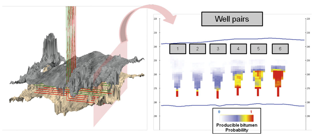
5. Finally, the proposed design, shown in Figure 8 (left) was validated in a 3D model displaying various confidence intervals of the position of top and base of the sands.

Connectivity and Ranking

Although this proposed pad is simplified, it can nonetheless be used as a starting point to quantify the vertical connectivity and to rank the 250 realizations using a criterion relevant to the SAGD production scheme. McLennan and Deutsch (2005) showed through flow simulation, that the oil production and the steam oil ratio are highly correlated to the volume of bitumen in the drainage volume. As a first approximation, the volume of bitumen that can be swept from a given producer well can be estimated by computing a simple steam chamber as an inverted triangle around that wellbore (Butler, 1991). These inverted triangles move upward from the well pairs and will be blocked or deviated by shale barriers. This producible volume was computed for each individual realization and by combining all the realizations, the probability of producible bitumen (Figure 8, right) could be generated. In this final step of the post-inversion analysis; the histogram of volume of sand connected to the producer(s) can be used to make better decisions in the light of the existing uncertainty (as it was for the length of the marine cable in the introduction). Using the criteria developed here, it was now possible to test different well locations and find better production zones.

This histogram of bitumen sand connected to the producers could also be used to rank the realizations. This ranking could be used to select individual realizations, typically a pessimistic, median and optimistic case (P10, P50 and P90) on which a more complete and realistic production and flow model may be built.

Conclusions

This workflow made improved use of seismic data in the characterization of heavy oil fields by systematically using probabilities or statistical criteria in order to quantify the uncertainties of each output.

It also enabled quick integration of well and seismic data in the elastic domain, providing reservoir parameters such as facies, flow barriers and connectivity; before any geomodeling was performed. Later the two flows could be merged, thus leading to potentially better models.

This type of workflow can be extended to other geological contexts, such as shale gas, where uncertainty in horizontal well positioning, reservoir qualities and connectivity are important.

Acknowledgements

The authors thank an anonymous client for permission to use their data, Dave Gray for fruitful discussions; also Graham Carter, Jon Downton, Brian Russell, Dan Hampson, Thierry Coléou, Bogdan Batlai and Philippe Doyen of CGGVeritas.