This is a continutation of Rock Physics of Geopressure and Prediction of Abnormal Pore Fluid Pressures Using Seismic Data (Part 1).
4. Seismic-to-pressure conversion
The sand/clay acoustic model for shaley sandstones, developed by Carcione et al. (2000) yields the seismic velocities as a function of clay (shale) content, porosity, saturation, dry-rock moduli, and fluid and solid-grain properties. As stated before, the large change in seismic velocity is mainly due to the fact that the dry-rock moduli are sensitive functions of the effective pressure, with the largest changes occurring at low differential pressures. The major effect of porosity changes is implicit in the dry-rock moduli. Explicit changes in porosity and saturation are important but have a lesser influence on wave velocities than changes in the moduli. This is due to the fact that the moduli are highly affected by the contact stiffnesses between grains. In this sense, porosity-based methods can be highly unreliable.
In order to use the theory to predict pore pressure, we need to obtain the expression of the dry-rock moduli versus effective pressure. The calibration process should be based on well, geolvogical and laboratory data, mainly sonic and density data, and porosity and clay content inferred from logging profiles.
Let us assume a rock at depth z. The lithostatic or confining pressure can be obtained by integrating the density log. We have that

where ρ is the density and g is the acceleration of gravity. Furthermore, the hydrostatic pore pressure is approximately given by ph = gρwz, where ρw is the density of water. As a good approximation (Prasad and Manghnani, 1997), compressional and shear-wave velocities and bulk and shear moduli depend on effective pressure pe = p – np, where p is the pore pressure and n is the effective stress coefficient, which can be different for velocities and moduli. Note that the effective pressure equals the confining pressure at zero pore pressure.
In general, n is approximately linearly dependent on the differential pressure pd = pc – p in dynamic experiments (Gangi and Carlson, 1996; Prasad and Manghnani, 1997). Therefore, we assume n = n1 – n2pd = n1 – n2(pc – p). This dependence of n versus differential pressure is in good agreement with the experimental values, corresponding to the compressional velocity obtained by Christensen and Wang (1985) and Prasad and Manghnani (1997). It is clear that to obtain n1 and n2, we need two evaluations of n at different pore pressures, preferably a normally pressured well and an overpressured well. If one well or equally pressured wells are available, the algorithm provides an average value for n.
Calibration of the model
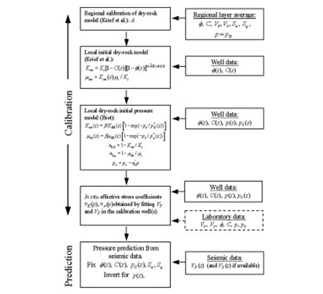
Ideally, a precise determination of n requires laboratory experiments on saturated samples for different confining and pore pressures. However, even this “laboratory” n does not reflect the behaviour of the rock at the in-situ conditions, due to two main reasons. First, laboratory measurements of wave velocity are performed at ultrasonic frequencies, and second, the in-situ stress distribution is different from the stress applied in the experiments. In the absence of laboratory data, or for shales, we perform the following steps with the data available from a calibration well (see Figure 4.2):
- We use Krief et al.’s model (Krief et al., 1990) modified by Goldberg and Gurevich (1998) to obtain the dry-rock moduli as a function of depth, using the clay-content and porosity profiles.
- We calculate the upper limit of the dry-rock moduli — at infinite effective pressure — using the Hashin-Shtrikman (HS) upper bounds (Hashin and Shtrikman, 1963), and assume an exponential law for the bulk moduli versus effective pressure.
- We compute the exponential coefficients (see equation (4.3)) using the values of the moduli obtained in step 1, the confining and (measured) pore pressures, and the effective stress coefficients predicted by Biot’s theory.
- We obtain the in-situ effective stress coefficients by fitting the theoretical wave velocities (Carcione et al., 2000) to the soniclog wave velocities, using the dry-rock moduli versus effective pressure obtained in steps 2 and 3, and n as a fitting parameter. The effective stress coefficient versus pore pressure, corresponding to the same geological unit, is obtained by using the linear law n = n1 – n2pd.
It is important to point out here that the HS bounds and Biot’s effective stress coefficient do not depend on the size and shape of the grain and pores. In this sense, the model has a general character. The only conditions are linearity, isotropy and the low-frequency approximation.
If sandstone cores are available, we proceed as follows:
- The upper limits (infinite confining pressure) and exponential coefficients of the moduli are obtained by fitting the dry-rock moduli, which are calculated from the dry-rock wave velocities, while n is obtained from experiments on saturated samples for different confining and pore pressures (Carcione and Gangi, 2000a,b).
- Continue with step 4 of the preceding list. This step should improve the determination of n, estimated with laboratory experiments in step 1.
More precisely, we use the following data of the study area, to calibrate the model and obtain the effective-stress-coefficient profile for the formations under consideration:
- An estimation of the porosity profile, ϕ(z) , to use in Krief et al’s model (see below) and in the sand/clay acoustic model (from a series of logs using artificial neural networks (Helle et al, 2001)).
- An estimation of the clay-content profile C(z), to use in Krief et al’s model (see below) and in the sand/clay acoustic model (shale volumes obtained from well logs using neural networks (Helle et al., 2001)).
- Direct measurements of pore pressure, p(z) from repeat formation tests (RFT) and/or mud weights provided by the mudlogging operator).
- Sonic-log information, that is, the P-wave and S-wave velocity profiles, VP(z) and VS(z), used to obtain nK and nμ for the whole range of effective pressures by fitting the theoretical wave velocities to VP and VS. Here, nK and nμ are the effective stress coefficients corresponding to the dry-rock bulk and shear moduli, respectively.
No laboratory experiments available
Firstly, we consider the model of Krief et al. (1990), to obtain an estimation of the dry-rock moduli, Ksm , μsm (sand matrix), and Kcm, μcm (clay matrix) versus porosity and clay content. The porosity dependence of the sand and clay matrices should be consistent with the concept of critical porosity (Mavko et al., 1998, p. 244) since the moduli should vanish above a certain value of the porosity (usually from 0.4 to 0.5). This dependence is determined by the empirical coefficient A (see equation (4.2)). This relation was suggested by Krief et al. (1990) and applied to sand/clay mixtures by Goldberg and Gurevich (1998). The bulk and shear moduli of the sand and clay matrices are respectively given by
where Ks and μs are the bulk and shear moduli of the sand grains, and Kc and μc those of the clay particles. Krief et al. (1990) set the A parameter to 3 regardless of the lithology, and Goldberg and Gurevich (1998) obtain values between 2 and 4, while Carcione et al. (2000) use A = 2. Alternatively, the value of A can be estimated by using regional data from the study area. We use a general form of Goldberg and Gurevich’s equation. Experimental data is fitted in Carcione et al. (2000), showing that the model has been successfully tested. The model is not based on a dual porosity theory, but there is only one (connected) porosity. The clay moduli are taken from fit to experimental data in Goldberg and Gurevich’s paper.
Secondly, we assume the following functional form for the dry-rock moduli as a function of effective pressure:

where α(z), and p*(z) should be obtained (for each moduli) by fitting Krief et al’s expressions (4.2). The effective pressure at depth z is assumed to be pe = pc – n0p, where pc is given by equation (4.1), p is given, and n0 is a first estimation of the effective stress coefficient, based on Biot’s theory (Todd and Simmons, 1972; Zimmerman, 1991, p. 33).
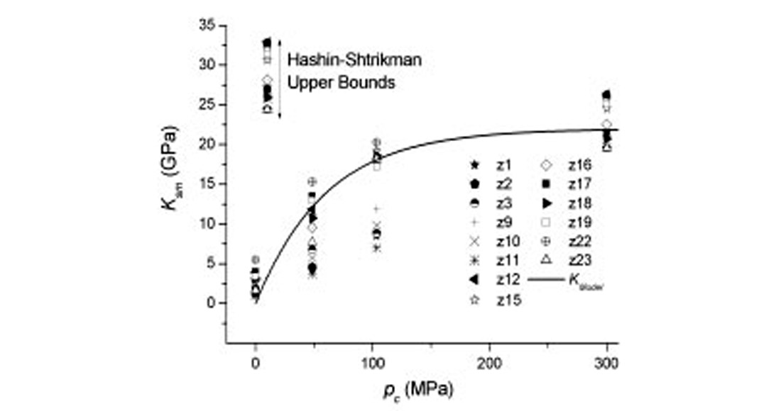
Since there are two unknown parameters (α(z), and p*(z)) and one value of M for each depth, α(z) is assumed to be equal to the Hashin-Shtrikman (HS) upper bounds (Hashin and Shtrikman, 1963, Mavko et al., 1998, p.106). Note that the HS lower bounds are zero, and that the Voigt bounds are (1 – ϕ) Ks and (1–ϕ)μs, respectively. For quartz grains with clay, Ks = 39 GPa and μs = 33 GPa (Mavko et al., 1998, p. 307), and if the limit porosity is 0.2, the HS upper bounds for the bulk and shear moduli are 26 GPa and 22 GPa, compared to the Voigt upper bounds 31 GPa and 26 GPa, respectively. However, the HS bounds are still too large to model the moduli of in-situ rocks. These contain clay and residual water saturation, inducing a chemical weakening of the contacts between grains (Knight and Dvorkin, 1992; Mavko et al., 1998, p. 203).
Figure 4.1 shows the dry-rock bulk modulus of several reservoir rocks for different confining pressures (Zimmerman, 1991, p. 29, Table 3.1), compared to the HS upper bounds. The solid line represents the analytical curve (4.4). On the basis of these data we apply a constant weight factor β = 0.8 to the HS bounds — due to the softening effects.
Equation (4.3) for the sand matrix can be written as

and

where we assume that the effective stress coefficients are given by Biot’s expressions (Todd and Simmons, 1972),
and pe depends on the specific coefficient. The last equality results from the third equation(4.2), and the second equation is merely an extension of the first to the case of shear deformations.
Laboratory experiments available
The evaluation can be improved if laboratory data of dry-rock P-wave and S-wave velocity are available, and serves to constrain the values of α and p* in equation (4.3). These sparse calibration points are based on sandstone or shaley sandstone cores, since dry measurements in shales are practically impossible to perform. The seismic bulk moduli Ksm and μsm versus confining pressure can be obtained from laboratory measurements in dry samples. If VP(dry) and VS(dry) are the experimental compressional and shear velocities, the moduli are given approximately by
where ρs is the grain density. We recall that Ksm is the rock modulus at constant pore pressure, i.e. the case when the bulk modulus of the pore fluid is negligible compared with the dry-rock bulk modulus, as for example air at room conditions. Then, we perform experiments on saturated samples for different confining and pore pressures, to obtain the effective stress coefficient n. Because these experiments yield the P-wave and S-wave velocities, and the effective stress coefficients of wave velocity and wave moduli may differ from each other, we obtain n for

where K and μ are the undrained moduli.
Calculation of the effective stress coefficients
The last step of the calibration process is to consider equation pe = pc – np and obtain the effective stress coefficients nK(z) and nμ(z) by fitting the theoretical velocities to the corresponding sonic-log P-wave and S-wave velocities, by using expressions (4.3). First, we obtain nμ by fitting the S-wave velocity, because this velocity only depends on μsm, and then, we obtain nK by fitting the P-wave velocity. If shear-wave velocity data is not available, we assume nμ = n0μ, i.e., the Biot estimate. From the values of n obtained at the two wells, we obtain the linear law for the geological unit under investigation. The values of clay content and porosity away from the wells are assumed to be equal to those of the nearest well. Interpretation is required to follow the geological units laterally, as a function of depth, so that the n profiles can be properly extrapolated. In this study, the clay-matrix modulus is simply given by Krief et al’s expressions, respectively, with no explicit dependence on pressure.
Pore-pressure calculation
Finally, the seismic velocity, derived from velocity analysis and inversion techniques, can be fitted with the theoretical velocities by using the pore pressure as fitting parameter. The theory (Carcione et al., 2000) allows us to introduce different kinds of information explicitly, such as composition (clay content), fluid saturation, porosity, permeability and viscosity (Pham et al., 2002). Before dealing with the seismic data we should test the above procedure in a nearby over-pressured well. The pore pressure prediction flow chart is shown in Figure 4.2 (Carcione et al., 2001, 2002).
AVO-based verification
In some cases, velocity information alone is not enough to distinguish between a velocity inversion due to overpressure and a velocity inversion due to pore fluid and lithology (e.g., base-of-salt reflections (Miley, 1999; Miley and Kessinger, 1999)). There are cases, where overpressuring is not associated with large velocity variations, as in smectite/illite transformations. Best et al. (1990) use AVO analysis to treat these cases. Modeling analysis of AVO signatures of pressure transition zones are given in Miley (1999), Miley and Kessinger (1999), Carcione (2000a,c) and Tinivella et al. (2001). This type of analysis should complement the present prediction method on the basis of geological information of the study area.
5. Application to a North Sea gas field
We consider the Tune Field area in the Viking Graben of the North Sea. This basin is 170-200 km wide, and represents a fault-bounded north-trending zone of extended crust, flanked by the mainland of western Norway and the Shetland platform. The area is characterized by large normal faults with north, northeast and northwest orientations which define tilted blocks. Such blocks contain the sequences present within the well used for this study. The main motivation for selecting this area is the fact that highly overpressured compartments were identified by drilling, and that higher overpressure is expected in future wells down the flank side towards the central Viking Graben. A detailed analysis of the fault sealing and pressure distribution in Tune Field is given by Childs et al. (2002).
Figure 5.1 displays a structural time map of Top Ness, showing the pressure compartments and the locations of three wells. Well 2 and 3 are overpressured (by about 15 MPa) and well 1 has almost normal (hydrostatic) pore pressure. The dashed line indicates the location of the seismic section shown in Figure 5.2. The calibration well (well 1) is an exploration well drilled to a depth of 3720 m (driller’s depth) to test the hydrocarbon potential of the Jurassic Brent Group. The well includes reservoir rocks of the Tarbert and Ness formations. The Tarbert sands are the target units considered in the present study.
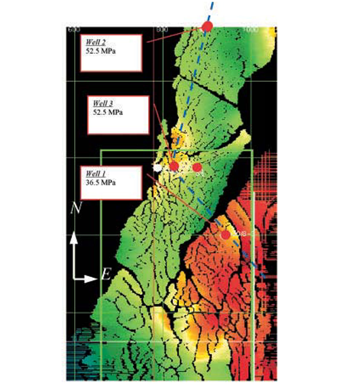
The 3-D marine seismic data was acquired by using a system of 6 streamers of 3 km length with a group interval of 12.5 m and cross-line separation of 100 m. The shot spacing was 25 m and the sampling rate 2 ms. The conventional stacked section is displayed in Figure 5.2, where the location of the wells is shown.
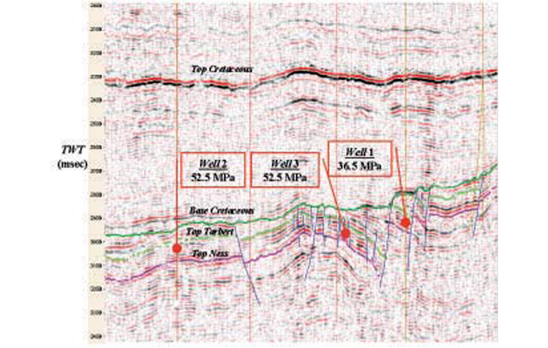
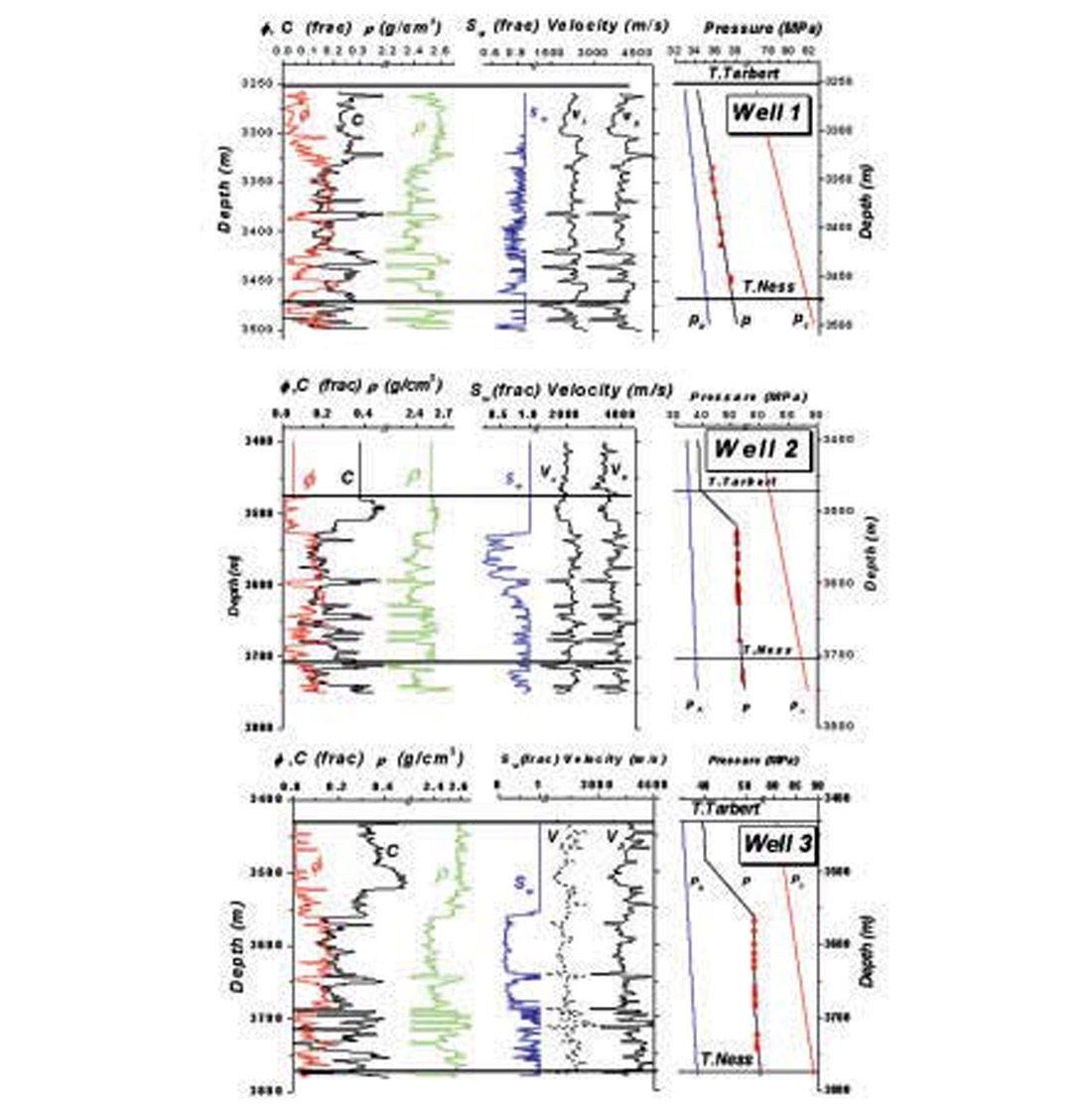
Figure 5.3 shows pressure and formation data (porosity ϕ, clay content C, density ρ, water saturation Sw and sonic-log velocities VP and VS) for the Tune wells. Note that well 1 is water bearing with moderate pore pressures while wells 2 and 3 are gas bearing and overpressured. Reservoir properties and fluid saturation are derived from wireline data using the neural net approach of Helle et al. (2001) and Helle and Bhatt (2002).
Velocity determination by tomography of depth migrated gathers
Recent advances in depth migration have improved subsurface model determination based on reflection seismology. Subsurface imaging is linked to velocity, and an acceptable image can be obtained only with a highly accurate velocity field. It has been recognized that prestack migration is a powerful velocity analysis tool that yields better imaging results than poststack migration in complicated structures. The basic assumption underlying the velocity determination methods based on prestack migration is that when the velocity is correct, all the migrations with data in different domains (e.g. different offset, different shots, different migration angles etc.) must yield a consistent image. In order to obtain the velocity field, we use the seismic inversion algorithm described by Koren et al. (1998).
We start with an initial model based on the depth converted time model, using a layer velocity cube based on conventional stacking velocities, and the interpreted timehorizons from the Tune project. Line by line, we perform the 3-D prestack depth migration using the initial velocity model and an appropriate aperture (3 km x 3 km at 3 km depth) in the 3-D cube. Through several iteration loops the model is gradually refined in velocity and hence depth. Each loop includes re-interpretation of the horizons in the depth domain, residual moveout analysis and residual moveout picks in the semblance volume. This is performed for each reflector of significance, starting at the seabed and successively stripping the layers down to the target.
The tomography considers, 1) an initial velocity model and, 2) the errors as expressed by the depth gather residual moveout and the associated 3-D residual maps. From these two inputs a new velocity model is derived where the layer depths and layer velocities are updated iteratively in order to yield flat gathers. The refined model is derived using a tomographic algorithm that establishes a link between perturbation in velocity and interface location, and traveltime errors along the common reflection point (CRP) rays traced across the model. CRP rays are ray pairs that obey Snell’s law and emanate from points along the reflecting horizon, arriving at the surface with predefined offsets, corresponding to the offset locations for the migrated gathers. Each pair establishes a relationship between the CRP and the midpoint of the rays at the surface. Depth errors, indicating the difference in depth of layer images and reference depth, are picked on the migrated gather along the horizon and converted to time errors along the CRP rays. The equations relating the time errors to changes in the model are solved by a weighted least squares technique.
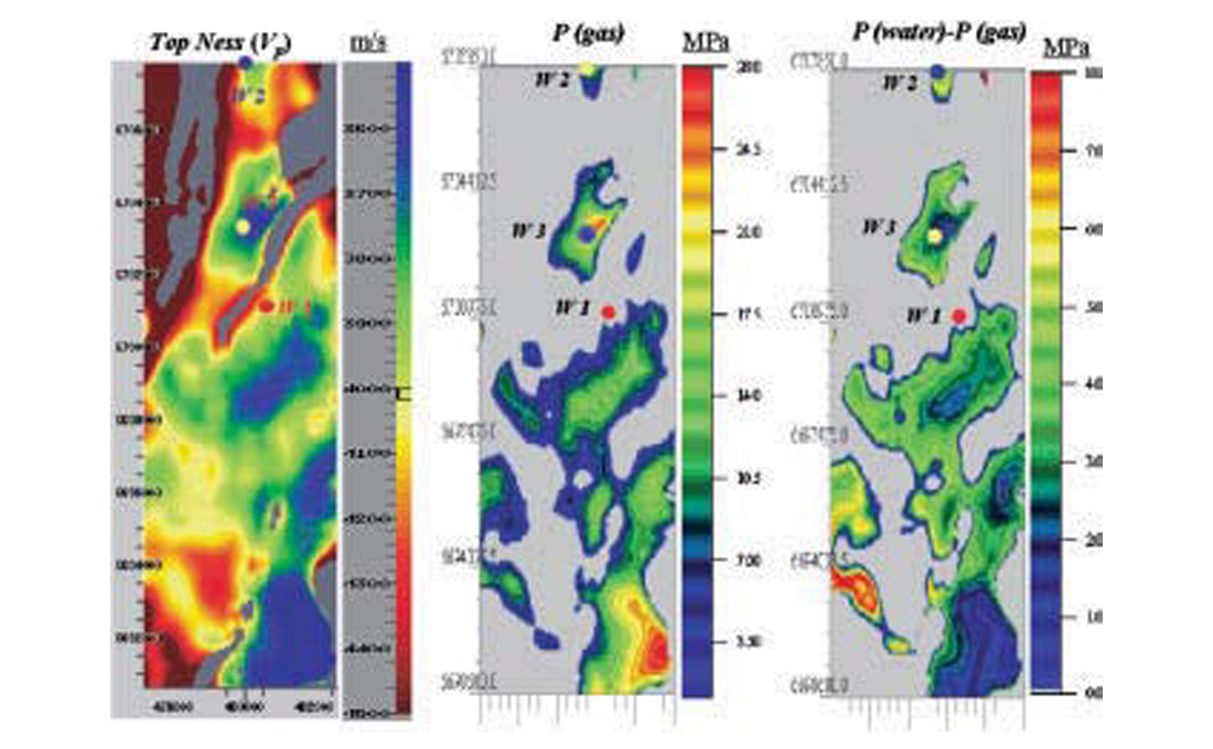
The final model consists of seven layers, i.e., the sea water layer, seabed-Top Diapir (clay diapirism is a characteristic feature of Tertiary throughout the area), Top Diapir-Top Balder, Top Balder-Top Cretaceous, Top Cretaceous-Base Cretaceous, Base Cretaceous-Top Tarbert, and the target layer, Top Tarbert-Top Ness. The velocity maps for Top Tarbert -Top Ness is shown in Figure 5.4 (left panel), where the well locations are indicated. The Cretaceous layer velocity and the depth to Base Cretaceous reveal a remarkable similarity, i.e., where the Cretaceous is deep the velocity is high and where the Cretaceous is shallow the velocity is low, indicating that the velocity of Cretaceous is essentially governed by the overburden (e.g. compaction). Base Cretaceous, Top Tarbert and Top Ness depth maps display the more dramatic geometry of Upper Jurassic, where the Tarbert Formation is completely eroded in the northwest and where patches of missing Ness are present along the major faults. These erosion features are, of course, well reflected in the layer velocities since here the layer thickness tends to zero and layer velocity is hence not defined. Structural features are well displayed in the velocity maps of the Top Tarbert and Top Ness. The Base Cretaceous- Top Tarbert velocity map reveals, however, a fairly scattered distribution, with small patches of highs and lows within the main fault blocks.
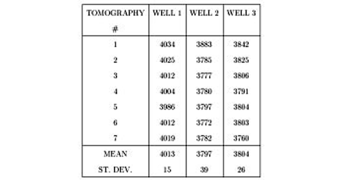
For the reservoir itself, represented by the Top Ness velocity map, the distribution is far more coherent. In the Tarbert formation at wells 2 and 3 in the North fault block, there are consistently lower velocities than at well 1 in the East block. This feature is fairly constant for several independent velocity analysis, with a velocity increase of about 200 m/s across the fault separating the gas-bearing reservoir in the North block from the water-bearing reservoir in the East block. A high-velocity ridge separates the lows at well 2 and 3. Distinct low-velocity zones are also seen to the south and southeast that are not correlated with the depth variations. On the other hand, the high-velocity zones in the southwest may be related to the Tarbert dipping down at the western flank. Table 5.1 shows the results of seven independent velocity analysis obtained in the three well locations, revealing that the differences in mean velocity between the “normal” well 1 and the two overpressured wells 2 and 3 are far beyond the estimated error.
Application of the velocity model for pressure prediction
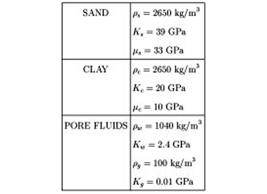
In order to estimate the pressure map in the Tarbert formation, we follow the procedure outlined above. Table 5.2 shows the values of the basic physical quantities used to compute the theoretical velocities. Gas density and gas bulk modulus are computed by using the van der Waals equation, as described in Carcione and Gangi (2000b). (The values indicated in the table are for hydrostatic pressure.) We assume, according to Biot’s theory, that n1 = 1, i.e., that at zero differential pressure the frame bulk modulus vanishes. The same assumption has been used for the effective stress coefficient related to the frame rigidity modulus. Figure 5.4 shows the velocity map (left panel) and the overpressure map assuming Sw = 0.35 and a gas saturation Sg = 0.65 (center panel). The picture at the right represents the difference in pore pressure by assuming gas-bearing Tarbert (the center picture) and water-bearing Tarbert (Sw= 0.94 and Sg = 0.06). An overpressure of about 15 MPa is predicted for well 2, while slightly higher overpressure (18 MPa) is predicted for well 3. The direct measurements indicate overpressures of about 15 MPa (see Figure 5.3). Figure 5.4 (right panel) shows that the sensitivity of the model to fluid saturation is about 8 MPa, indicating that significant uncertainity can be attributed to assumption of uniform saturation.
The velocity obtained by careful analysis of pre-stack 3-D data from the deep and complex Tarbert reservoir in the Tune gas field is sufficiently sensitive to pressure and pore fluid to perform a meaningful analysis. The velocity and pressure distribution complies well with the structural features of the target and the general geological understanding of the pressure compartments in the Tune field. The partial saturation model used for pressure prediction can conveniently be calibrated against well data, provided that a complete set of logging data are available for the zone of interest. The most important part of the prediction process is the determination of the effective stress coefficients and dry-rock moduli versus effective pressure, since these properties characterise the acoustic behaviour of the rock. The inversion method based on the shaley sandstone model must fix some parameters while inverting the others. For instance, assuming the reservoir and fluid properties (mainly, the saturation values), formation pressure can be inverted. Conversely, assuming the pore pressure, the saturations can be obtained. The latter implies that this method may be used in reservoir monitoring where the pressure distribution is known while saturation, i.e., the remaining hydrocarbon reserves, are uncertain. We have neglected velocity dispersion, which is not easy to take into account, since Q factor measurements are rare and difficult to obtain with enough reliability. When using laboratory data for the calibration, the effect of velocity dispersion can be significant (Pham et al., 2002).
6. Conclusions
Abnormal pressure, or pressures above or below hydrostatic pressure, occurs on all continents in a wide range of geological conditions. In young (Tertiary) sequences, compaction disequilibrium is the dominant cause of abnormal pressure. In older (pre-Tertiary) rocks, hydrocarbon generation and tectonics are most often cited as the causes of overpressure. Hydrocarbon accumulations are frequently found in close association with abnormal pressure. Thus, in exploration for hydrocarbons and exploitation of the reserves, knowledge of the pressure distribution is of vital importance for prediction of migration routes and location reserves, for the safety of the drilling and for optimising the recovery rate in production.
In this study, we have quantified the effect on seismic properties caused by the common mechanisms of overpressure generation such as hydrocarbon generation, oil-to-gas cracking and disequilibrium compaction. Fluid pressure due to hydrocarbon generation in source-rock shale significantly reduces the seismic velocities and enhances the anisotropy. Attenuation and attenuation anisotropy are also strongly effected, thus further enhancing the seismic visibility of overpressure in the shale. In deeply buried reservoirs, oil-to-gas cracking may increase the fluid pressure to reach lithostatic pressure, and the seismic velocities are shown to drop significantly when only a small fraction of oil in a closed reservoir is converted to gas. Non-equilibrium compaction generates abnormal pressures that, under certain conditions, can be detected with seismic methods. In this case, the fluid mixture filling the pore-space has a major influence on P-wave velocity and my cause under- or over-pressures depending on its compressibility and thermal expansion coefficient. Rocks saturated with fluids of low compressibility and high thermal expansion are generally overpressured and can be seismically visible.
The feasibility of pressure prediction from seismic data rely upon two main factors:
- Accuracy of the relationships linking the rock physics parameters to pore pressure and properties of the seismic wavefield.
- The quality of the seismic data and the analysis of seismically derived parameters such as the wave velocity and amplitude (AVO).
We have attempted to link the rock physics parameters, based on first-principles, directly to pore pressure whereas the common conversion methods are based on empirical porosity-stress models valid only for shales saturated with water. Our method, on the other hand, applies to shaley reservoir rocks as well as pure sandstone and shale. Since drilling hazard more often is associated with overpressure in reservoir rocks containing gas rather than with low-permeability water saturated shale, a more general method that accounts for variation in lithology and pore-fill can be justified. However, no reliable method of pore pressure estimation from seismic data can be applied without model calibration against rock physics parameters, as obtained from well logs or laboratory experiments. In absence of local wells a calibration based on regional data is normally in favour of importing empirical relationships developed for a different basin.
Recent developments in 3-D seismic data acquisition and processing techniques have provided an appropriate platform for accurate estimation of seismic velocity and amplitude for input to the pressure analysis. This is further fertilised by the recent developments in techniques and availability of software for 3-D prestack depth migration, velocity tomography and AVO, which greatly enhance the feasibility of pore pressure estimation from seismic data.
The velocity obtained from the Tune gas field is sufficiently sensitive to pressure and pore fluid to perform a meaningful analysis. A critical step in the prediction procedure is the determination of the effective stress coefficients and dry-rock moduli versus effective pressure, since these properties characterise the acoustic behaviour of the rock. The inversion method based on the shaley sandstone model must fix some parameters while inverting the others. For instance, assuming the reservoir and fluid properties, formation pressure can be inverted. Conversely, assuming the pore pressure, the saturations can be obtained. The latter also illustrates the ambiguity imbedded in the problem that may be resolved by AVO.

Acknowledgements
The European Union under the project “Detection of overpressure zones by seismic and well data” has supported a substantial part of this work.


Join the Conversation
Interested in starting, or contributing to a conversation about an article or issue of the RECORDER? Join our CSEG LinkedIn Group.
Share This Article