Robust Workflows for Seismic Reservoir Characterisation

In the talk I describe a workflow for seismic reservoir characterisation. The specific problem I address is the estimation of net-to-gross from a clastic reservoir, however the workflow is adaptable for a variety of other applications.

The three main components of the workflow are:

1. Extended elastic impedance analysis followed by 2-term AVO coordinate rotation of the seismic intercept and gradient datasets.
2. Coloured inversion.
3. Attribute extraction followed by calibration and detuning.

This workflow has evolved within BP over the past decade or so. The component processes are all fundamentally very simple; they all operate within the seismic bandwidth (other than the initial well data analysis) and the number of parameters required to implement them is small. This leads to a very robust workflow; the subjectivity of the parameter selection is minimised so the results tend to be repeatable.

Extended Elastic Impedance

Extended elastic impedance is based on the gradient impedance/ acoustic impedance crossplot domain (Whitcombe & Fletcher, 2001). Gradient impedance (GI) is a function of Vp, Vs and density, with associated reflectivity equal to the gradient term in the 2-term AVO equation. Extended elastic impedance (EEI) (Whitcombe et al, 2002) is a coordinate rotation in AIGI space (using log-log axes). An EEI curve is parameterised by the rotation angle, chi.

The chi angle can be selected to optimise the correlation of the EEI curve with a target reservoir parameter such as VShale or porosity or with an elastic parameter such as bulk or shear modulus, Poisson’s ratio or shear impedance.

The equivalent process can then be performed on seismic data by combining intercept and gradient datasets using the same coordinate rotation weightings (Hendrickson, 1999). In practice for a number of reasons the optimal seismic angle will probably be different from the optimum angle calculated from the log data so an additional optimisation process is required. The result is a seismic dataset with an optimum correlation with a desired parameter which can then form the basis for a reservoir characterisation workflow.

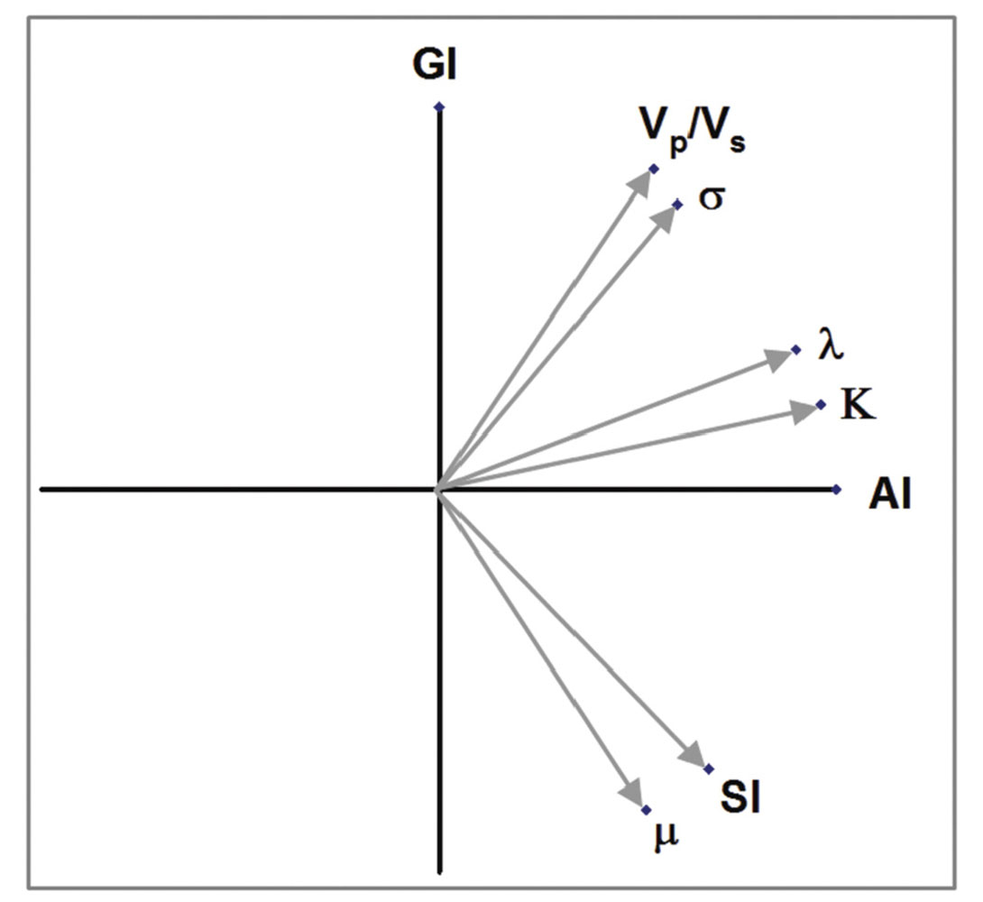
It has been recognised for some time that combinations of AVO parameters can provide useful approximations to a number of elastic parameters (Dong, 1996, Goodway et al, 1997). Any simple combination of intercept and gradient is equivalent to a coordinate rotation (figure 1). By performing this rotation in the impedance domain in intercept-gradient space the correlation coefficient between the EEI log and elastic parameter provides a quantitative assessment of the quality of the approximation. These approximations are often very good.

This approach can also be used to demonstrate the equivalence of different AVO domains. For example Poisson’s Ratio and shear impedance typically have high correlations at specific rotation angles within the AIGI domain implying that AIPR, AISI and AIGI domains are just stretched and squeezed versions of each other.

Coloured inversion

As much as we’d like to be able to invert our seismic data to absolute impedance in many circumstances the additional low frequency data required to do this is unreliable. A safer option is to base seismic characterisation on band-limited impedance. To transform seismic to band-limited impedance (BLI) we need to understand the characteristics of impedance amplitude spectra.

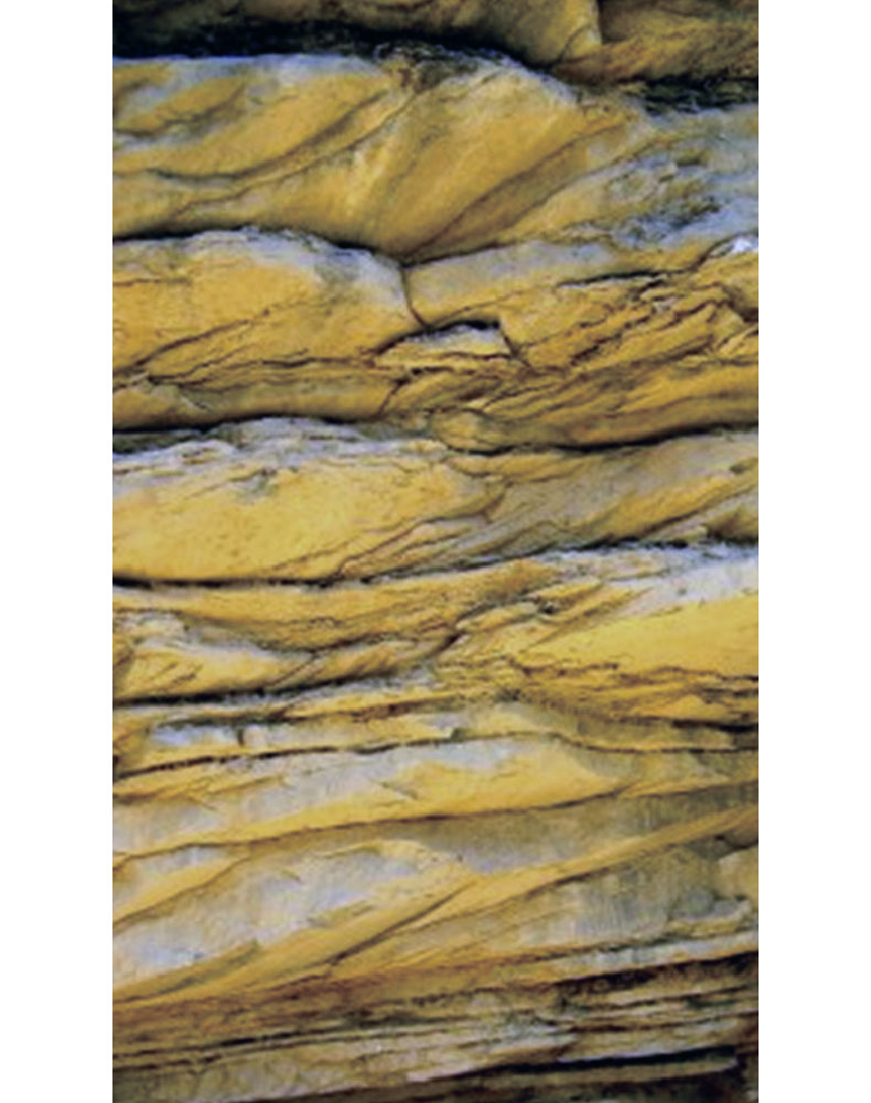
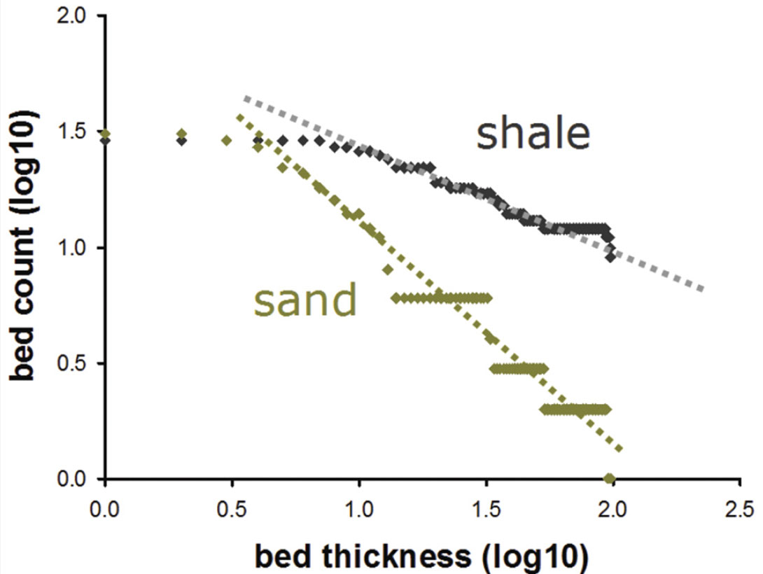
Geology has long been recognised as being, at not at least partially, scale invariant; photographs of outcrops require something to provide scale (figure 2). Mathematically this means that bed thickness distributions (figure 3) tend to follow a power law relationship (Talling, 2001) with the implication that say gamma ray curves are fractal. The importance of this for geophysicists is that fractal curves have power law amplitude spectra (Turcotte, 1997) and hence, because we’ve seen that impedance logs can be made to correlate with gamma ray curves, they too will have power law spectra (Stefani & De, 2001).

Coloured inversion (Lancaster & Whitcombe, 2000, Lancaster & Connolly, 2007) is the process to transform zero phase seismic data of arbitrary (but stationary) amplitude spectrum to bandlimited impedance having a power-law spectrum limited by the bandwidth of the seismic. This process will result in optimal resolution within a given bandwidth. It is also a very simple process requiring only an estimate of the power-law exponential from calibration well data and optimisation of the bandwidth.

Seismic net-to-gross

We can think of net-to-gross as being the ratio of the value of an average measurement, such as gamma ray, across the reservoir to the value of that measurement for the 100% net case (all measurements relative to the non-net baseline). If impedance correlates with GR the process will also work using an impedance log.

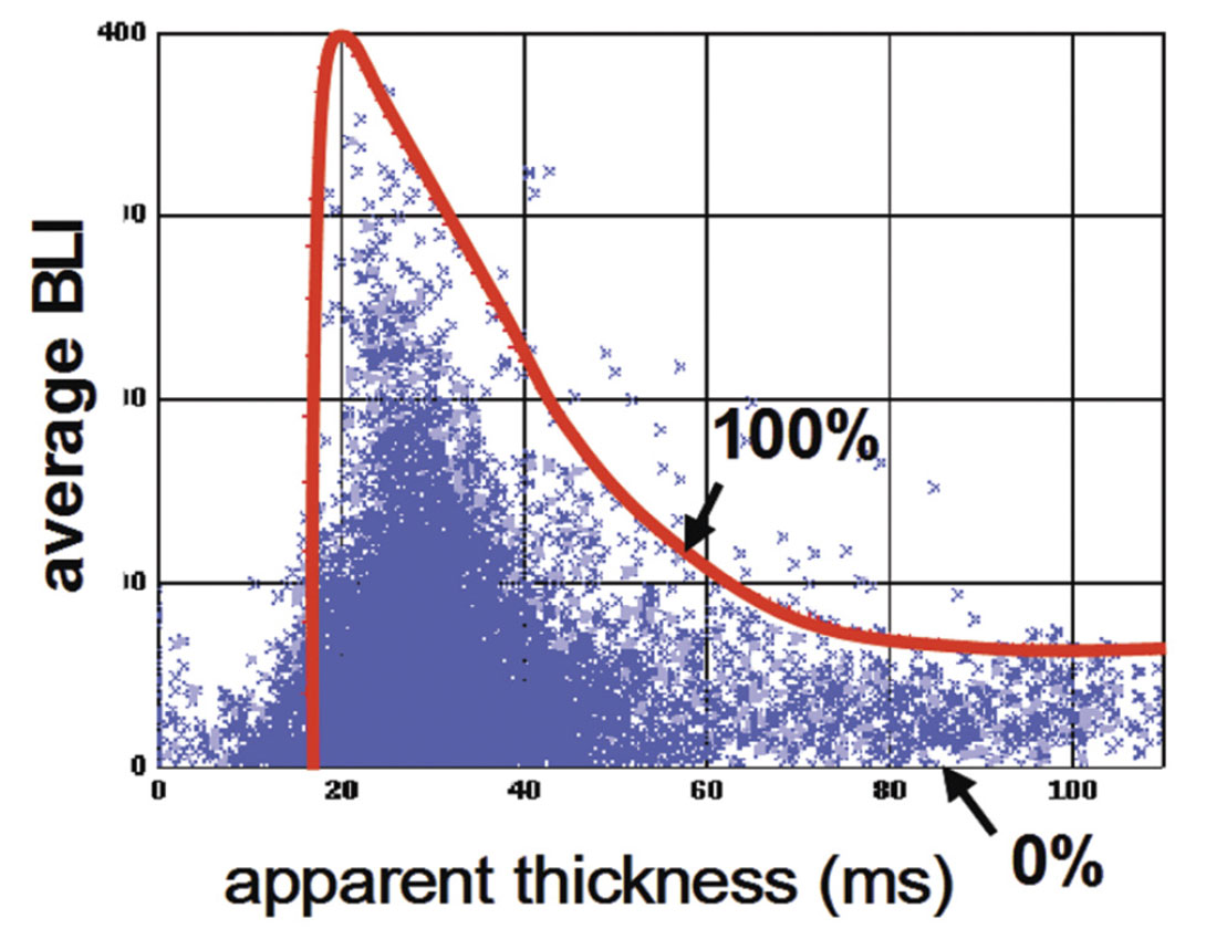
That concept can be extended to band-limited impedance. The 100% net value will now depend on gross thickness because of tuning effects but this can be modelled if we know the wavelet. The scaling of the tuning curve (figure 4) can be deduced either from geological insight (for example that the maximum net-togross of a turbidite reservoir is likely to be 100%) or by calibrating to well data (Connolly, 2007).

Seismic data that has been optimised to correlate with a gamma ray curve by using EEI analysis and then transformed to bandlimited impedance by coloured inversion can therefore provide a basis for net-to-gross estimation by a fairly simple detuning and calibration process. Provided apparent thickness is always used as the basis for the net-to-gross estimate the process remains consistent and works for sub-tuning as well as thicker reservoirs the maximum thickness being limited by the lack of low frequencies.

Robustness and uncertainty

The three processes in the workflow are all fundamentally simple. They each require a small number of parameters, which have fairly well defined methods of optimisation. This helps to make the workflow robust and repeatable. Minimising the subjectivity puts us in a position to consider making quantitative estimates of the uncertainty of our characterisation results; to put error bars on our reservoir predictions.

To do this we must consider the sources of uncertainty. I propose grouping these into three categories; geological uncertainty, calibration uncertainty and seismic uncertainty.

Geological uncertainty is caused by the sub-seismic scale variability in the rock properties and of the fine-scale layering. We can only estimate the impact of these effects statistically. One approach is to use pseudo-wells; a large number of geologically realistic synthetic wells constrained by calibration data. These can provide a statistical relationship between the seismic attribute and the required reservoir parameter (Connolly & Kemper, 2007).

Calibration uncertainty arises from the process of detuning and calibrating the seismic attributes. The level of uncertainty can be directly estimated and is dependent on the quality of the calibration data and the reliability and consistency of the wavelet estimation.

Seismic uncertainty is the inherent limited fidelity of the seismic amplitudes caused by the inability of the processing to fully correct for all the transmission effects, to remove all the noise and to perfectly image the data. Estimating the amplitude uncertainty is difficult but an indication of the level can be obtained by comparing independent surveys at the same location.

In principle each of these sources of uncertainty can be independently estimated and summed to provide an uncertainty map; in the example discussed this will be the standard deviation of the seismic net-to-gross. A capability to routinely do this would provide numerous benefits;

1. A better understanding of the relative size of different sources of uncertainty potentially leading to improvements in characterisation processes.
2. An ability to put meaningful errors bars on reservoir predictions.
3. The use of uncertainty maps to constrain reservoir modelling to ensure that models are consistent, but not driven by, the seismic data.

More fundamentally an ability to estimate uncertainty will allow us to better integrate different types of data and hence develop more accurate models of the subsurface.