Ricker, Ormsby, Klander, Butterworth – A Choice of Wavelets

Commercially available software used to generate synthetic seismograms gives the geophysicist a choice of up to four types of standardized wavelets as well as the option of a user-defined wavelet. This review article will summarize the characteristics of these wavelets, illustrate the shape of the wavelets and their frequency spectrum and present the parameters needed to define them as well as their mathematical formulas. In all the following formulas, "t" is time in seconds, "f" is frequency in hertz and "π" is the irrational number pi). Illustrations of the wavelets and their frequency spectrum were generated using the scientific numeric computation software MATLAB and the wavelets were chosen to have as similar a bandwidth as possible for ease of comparison.

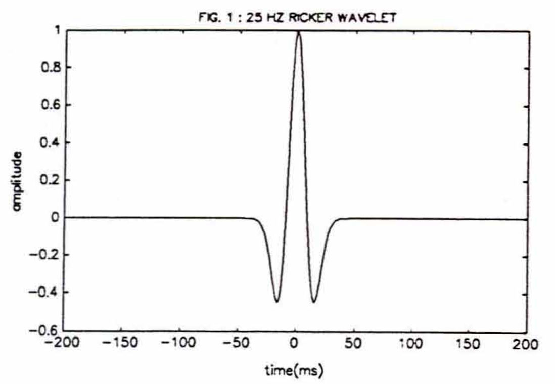
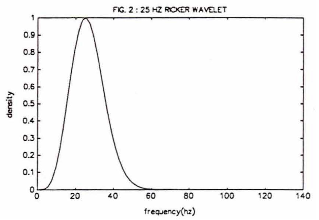
Ricker wavelets (fig 1) are zero-phase wavelets with a central peak and two smaller side lobes. A Ricker wavelet can be uniquely specified with only a single parameter,"f", it's peak frequency as seen on the wavelet's frequency spectrum (fig 2). The mathematical formula for a Ricker wavelet is given by:

In some texts you will see the Ricker wavelet's breadth, that is the time interval between the centre of each of the two side lobes, quoted as the reciprocal of the Ricker wavelet's peak frequency. This is only an approximation and indeed will give a wavelet breadth 28% wider than the true wavelet breadth. The correct formula for the breadth of a Ricker wavelet is:

Because of the simple inverse relationship between the peak frequency and breadth of a Ricker wavelet, the same Ricker wavelet could be just as uniquely described as a "31 ms Ricker wavelet" or as a "25 Hz Ricker wavelet".

Ormsby wavelets are also zero-phase wavelets although Ormsby, an aerospace engineer, actually defined a filter so such wavelets should really be called Ormsby-filtered wavelets. The trapezoidal shape of an Ormsby filter can be seen in the frequency spectrum shown in figure 4. Applying this filter to a unit impulse function results in the creation of the Ormsby wavelet shown in figure 3. An Ormsby wavelet will have numerous side lobes unlike the simpler Ricker wavelet which will always only have two side lobes.

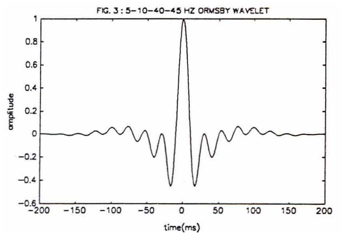
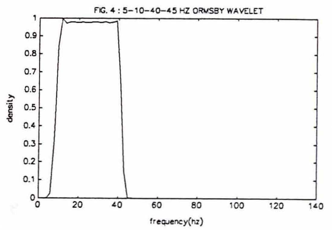
The Ormsby wavelet will also become more leggy the steeper the slope of the sides of the trapezoidal filter. Four frequencies are needed to specify the shape of an Ormsby filter and which are also used to identify an Ormsby wavelet (i.e. the 5-10-40-45 Hz Ormsby wavelet of fig. 3). These frequencies are "f1", the low-cut frequency; "f2", the low-pass frequency; "f3", the high-pass frequency and "f4", the high-cut frequency which are all used in the following formula to generate an Ormsby wavelet:

Like Ricker and Ormsby wavelets, a Klauder wavelet (fig 5) is symmetrical about a vertical line through its central peak at time zero. A Klauder wavelet represents the autocorrelation of a linearly swept frequency- modulated sinusoidal signal used in Vibroseis. It is defined by its terminal low frequency, "f1"; its terminal high frequency, "f2"; and the duration of the input signal "Τ", often 6 or 7 seconds. The real part of the following formula will generate a Klauder wavelet:

The frequency spectrum of a Klauder wavelet (fig 6) clearly shows the substantial similarities between a Klauder and an Ormsby wavelet.

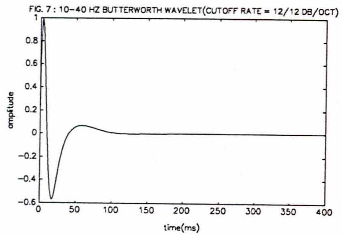
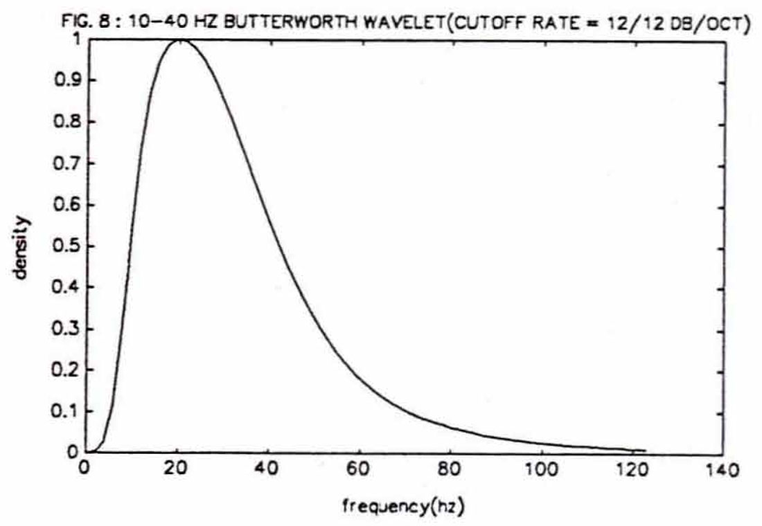
The most distinctive characteristics of Butterworth wavelets is that they are minimum- phase and physically realisable. A Butterworth wavelet will start at time zero while Ricker, Ormsby and Klauder wavelets all have their peaks at time zero. Butterworth defined a minimum-phase filter with maximal flatness in the passband so that applying a Butterworth filter to a unit impulse function will generate a wavelet such as in figure 7. Four parameters are needed to specify a Butterworth filter, beginning with "f1" and "f2", the lower and upper frequencies of the bandpass. Then the lower and upper cutoff rates, that is the slope of the amplitude response outside the bandpass, are needed. They are expressed as either "n", the order of the Butterworth filter (a positive integer) or in terms of "decibels/octave" which is "6n" (i.e. the cutoff rate can be described as either "third order" or as "18 decibels/octave"). As the cutoff rate of a Butterworth filter increases, the wavelet itself becomes more leggy. In an article by Curtis (1975) there is an appendix entitled "Generation of a Wavelet from Butterworth Filter Spectral Characteristics" which provides a thorough mathematical treatment of Butterworth filters. MATLAB has the advantage of containing a function for Butterworth filter design in its signal processing toolbox so that Butterworth wavelets and their frequency spectrum (fig. 8) can be generated quite easily.

Every time a synthetic seismogram is generated, the geophysicist must first choose the type of wavelet that will be used and then the specific parameters needed to define the wavelet. Making these choices becomes much easier with a thorough understanding of the differences and similarities between Ricker, Ormsby, Klauder and Butterworth wavelets and how varying their parameters changes the shape of the wavelet and its frequency spectrum.