Regularized migration/inversion: New Generation of Seismic Imaging Algorithms

Abstract

Linearized seismic inversion demands minimizing a cost function of the form

where L denotes the forward modeling operator that maps an angle dependent reflection strength m to a measurable seismic wave field d. Minimizing the cost function J in a least-squares sense, leads to the so-called least-squares migration methods. Migration algorithms, on the other hand, are only capable of estimating a blurred version of m by using the adjoint operator L′ (or a modified version of it). Migration methods, in general, do not attempt to find an image that can be used to reconstruct the seismic data. Moreover, they have little control on the achievable resolution besides the one provided by the data. One way of improving resolution is by incorporating model space constraints. These constraints are utilized to force the solution to exhibit desirable characteristics. We discuss the implementation of quadratic and non-quadratic constraints, similar to those used in image processing, to generate images with enhanced lateral and vertical resolution. We also stress that these ideas are not completely new; they have been used in applied seismology to solve a variety of interesting problems: sparse-spike deconvolution for impedance inversion, high resolution Radon processing and, more recently, high resolution AVO analysis. These ideas are a consequence of our continued quest for methods that can deliver models and images with resolution beyond the natural resolution provided by the spatio-temporal bandwidth of the acquired seismic wave fields.

Introduction

Linearized inversion of seismic data calls for the solution of the following problem:

where d indicates the multi-source multi-receiver seismic data, m denotes an earth model that consists of physical model perturbations or an angle dependent reflectivity. The operator L is a linearized one-way forward modeling operator computed on a known background model (macro-model), and n denotes coherent plus incoherent noise. Unavoidable errors in the operator can also be absorbed in the noise term. The forward modeling operator is often called the de-migration operator.

Rather than attempting to invert L via direct (analytical) methods, it has been proposed to invert L using a fitting procedure like the least-squares method (Nemeth et al., 1999). What is the advantage of such a procedure? First, we can include data and model space penalty operators to minimize the influence of inadequate sampling, operator mismatch, and coherent noise. In other words, the problem can be treated as a Bayesian inference problem where a priori information about the unknown image and observations can be included and used to minimize unwanted artifacts. Secondly, weighting matrices in data space can be used to minimize the influence of missing observations.

Regularization

Before starting with our discussion, it is important to stress that many well-known seismic processing problems can be written as linear ill-posed problems like the one given by equation (1). A short introductory recount will serve to pose the problem and highlight the role played by regularization methods at the time of inverting linear operators.

Regularization methods provide a procedure to guarantee the stability and uniqueness of the solution of an inverse problem. In general, we minimize a cost function of the form:

The first term is the data misfit for a class of inference problems where we have considered Gaussian (and possible correlated) errors. The data covariance matrix can be replaced by an empirical expression that assigns errors in terms of the distribution of sources and receivers; in equation (2) W_d is a matrix of weights proportional to the inverse data covariance matrix. The latter, for instance, can be used to mitigate acquisition footprints in wave equation migration methods (Kuehl and Sacchi, 2001 and 2003). The second term in equation (2), R ( m ), is often called the regularization term. This term, when obtained via the Bayesian framework, is associated with the a priori distribution of model parameters m.

Quadratic regularization

Model parameters that are normally distributed and correlated lead to quadratic regularization terms of the form:

In general, it is possible to approximate the barely known structure of the covariance matrix by weighting matrices that control the generation of undesired features in the solution. For instance, one can penalize roughness by replacing W_m by a first or second order derivative operator. In other words, W_m can be replaced by a high-pass operator that enhances undesirable features of m prior to minimization. This leads to a solution where the so-called undesirable features (highly oscillatory model components) are minimized.

The minimizer of J is given by the least-squares solution with quadratic regularization:

Notice that in the particular case when the data and model space weights are the identity operators, equation (4) reduces to the damped least-squares solution

An interesting interpretation of the problem arises when considering a regularization term with W_m=1 (equation (5)). From a Bayesian point of view, this case coincides with the maximum a posteriori solution for a problem where both observational errors and model parameters are considered uncorrelated and normally distributed. Under these conditions, it can be shown that the trade-off μ represents a signal-to-noise figure of merit given by

In situations of low signal-to-noise-ratio μ >>1 which leads to the following approximation (L′L +μI)≈ μI, and therefore, after considering equation (5), to the following expression

The solution m′ does not fit the data in addition, expression (7) represents a safe low-resolution solution. In other words, there is no risk of noise amplification, there is, however, a consequential resolution degradation trade-off.

Non-quadratic regularization

Non-Gaussian a priori distribution of model parameters leads to non-quadratic regularization terms. For instance, if we assume that the elements of the model parameter vector m are modeled via a Cauchy probability density function (see for instance; Sacchi, 1997) the resulting regularization term is given by

The latter is the Cauchy regularization term proposed by Sacchi and Ulrych (1995) as a means to achieve high-resolution Radon panels for velocity analysis and the attenuation of multiple reflections. Alternatively, one could have adopted a double Laplace exponential probability density function as the a priori distribution of model parameters. The latter leads to a l₁ regularization term

Inversion with the Laplace regularization term R_L(m) is the basis of high-resolution sparse-spike inversion methods for impedance inversion (Oldenburg et. al, 1983).

Quadratic vs. Non-quadratic regularization applied to two classical problems

The diagram in Figure (1) highlights the use of quadratic and non-quadratic constraints in two classical inverse problems in seismic data processing: deconvolution and the design of Radon operators. In both cases, an important increment in resolution can be achieved by introducing non-quadratic regularization.

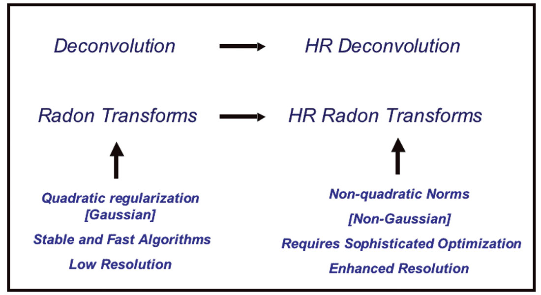
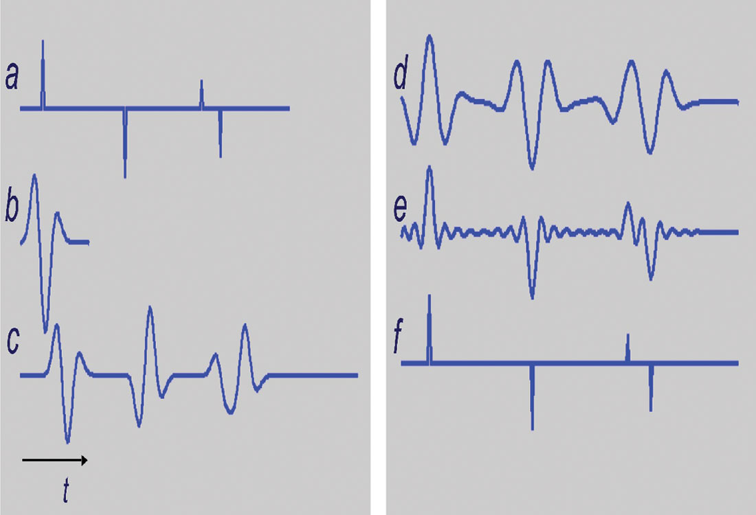
Figure 2 shows a simple deconvolution example. In this example, m represents the reflectivity sequence, d a zero-offset seismic trace, and L represents a wavelet matrix expressing time-invariant convolution. The reflectivity sequence (a) is convolved with a band-limited minimum phase wavelet (Figure 2 b), the resulting seismic trace is portrayed in Figure 2c. Figure 2d shows the cross-correlation of the seismic wavelet with the seismic trace. This is equivalent to processing the data with the adjoint operator L′ (Equation (7)). It is important to notice that the resolvable reflections are clearly recognizable, however, the two non-resolvable events are hard to recognize due to wavelet interferences. The least-squares solution with quadratic regularization is depicted in Figure 2e. We observe an important improvement in the resolution of the estimated reflectivity. In addition, the wavelet has been properly de-phased. There is, however, a bandlimited residual wavelet embedded in the estimator that can hamper subsequent processes that require full-band reflectivity estimates (e.g. impedance inversion). Finally, Figure 2f displays the deconvolution obtained via non-quadratic regularization (sparse-spike solution). In this particular case, a Cauchy regularization term was utilized to retrieve the full-band solution. This simple example shows an evolution of ideas that can be easily exported to other types of inverse problems. For instance, in the processing of seismic data with the Radon transform it has been noticed that quadratic regularization methods yield Radon panels that do not exhibit enough resolution to properly identify and separate multiples from primaries. The addition of non-quadratic constraints (Cauchy regularization) leads to high-resolution Radon operators (Sacchi and Ulrych, 1995).

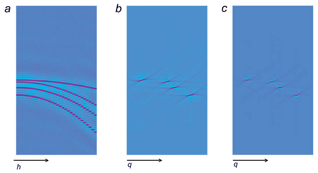
In Figure 3, we exemplify the problem with the Parabolic Radon transform but bear in mind that non-quadratic regularization methods can also be used to design high resolution hyperbolic Radon transforms (van Dedem, 2002; Trad et al., 2003) and high resolution Fourier interpolation/reconstruction methods (Sacchi et. al., 1998). Recently, non-quadratic Cauchy regularization strategies have been used for high resolution AVO analysis (Downton, 2005).

Regularized Inversion of the De-Migration Operator

We have seen that when the inverse of L represents a focusing operator that attempts to collapse a certain class of events to points (i.e., Radon operator), R(m) can be chosen to be a measure of sparseness (simplicity). Notice that in this case m does not have a direct physical interpretation. In this context, m does not represent a perturbation of physical properties, it is just a new domain where it is possible to isolate, and filter undesired waveforms.

Let us analyze the case where L represents a forward modeling operator that maps the distribution of physical properties to measurable seismic wave fields. In this case, a sparse solution is only valid for a subsurface model that consists of a sparse distribution of isolated scatterers. This might be a good framework for certain non-invasive imaging problems in material and medical sciences but not a realistic one for seismic exploration problems. In exploration seismology, we are interested in the distribution of the reflectivity as an expression of geological discontinuities. We expect a certain degree of spatial continuity of reflectors with well-defined vertical and horizontal scales. All the above is complicated by the addition of structural elements like faults, folds, and unconformities. Therefore it is clear that a regularization term capable of expressing desirable geological features will first involve obtaining quite an important amount of information about the unknown distribution of physical properties.

Avoiding the aforementioned shortcoming requires the parameterization of the seismic image m as an angle dependent reflectivity (de Bruin et al., 1990). As we will see in the next section, the latter simplifies the selection of the regularization term.

Migration and Inversion of angle dependent reflection strength

As we have stated in the introduction, we consider the seismic data as the result of a linear transformation d = L m + n , where d denotes the pre-processed data, L is the forward operator, m is the angle dependent reflectivity. Depending on the selection of the migration/de-migration algorithm, the angle dependent reflectivity can be parameterized in terms of offset (Duquet et al., 2000) or ray parameter. We use the ray parameter parameterization when working with wave equation de-migration/migration algorithms (Stolt and Weglein, 1985; de Bruin et al., 1990; Prucha et al., 1999; Kuehl and Sacchi, 2003).

Conventional migration entails applying L′, the adjoint of L, to the observed data. When the data are properly sampled, the migration amplitudes can be corrected by incorporating the Jacobian correction (Sava et al., 2001). This correction attempts to make the adjoint operator behave like the inverse operator. In general, the correction is not sufficient to achieve good amplitude fidelity. Sampling and migration artifacts are not suppressed by it. These artifacts can be attenuated, however, by constraining the solution to exhibit a certain degree of smoothness along the ray parameter axis. In this case, we adopt the following cost function to retrieve a migrated image that fits the observations and, in addition, exhibits smoothness or continuity along the ray parameter axis:

where W_p denotes a high-pass operator with respect to the ray-parameter axis. The latter leads to a solution where high ray parameter variability in the common image gathers is penalized. The diagram in Figure 4 summarizes the current state of affairs in imaging and regularized imaging. Algorithms based on the minimization of equation (10) have been reported by research groups (Kuehl and Sacchi, 2001 and 2003; Prucha-Clapp and Biondi, 2002). Our synthetic and field data examples were obtained with the algorithms described in Kuehl and Sacchi (2003), Wang et al., (2005) and Wang (2005). The de-migration operator is synthesized via a 3-D common azimuth wave equation propagator for complex media with the addition of a ray-parameter transformation to map subsurface wave fields to ray-parameter dependent reflectivity (Biondi and Palacharla, 1996; Prucha et. al, 1999).

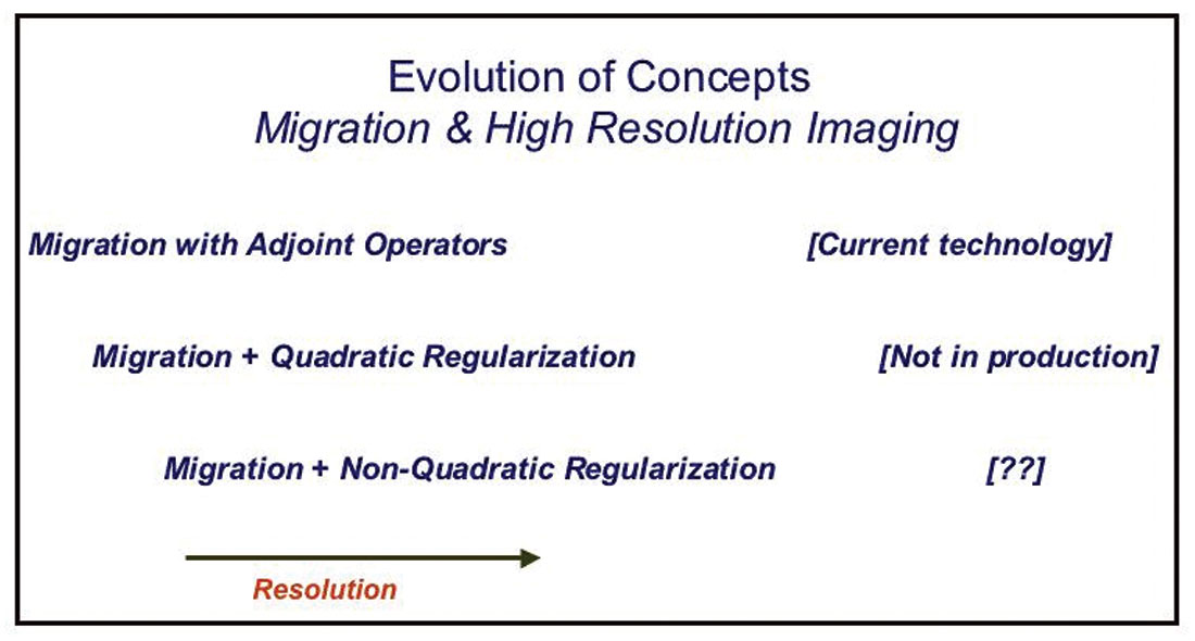
Figure 5 provides a common image gather computed using migration (Figure 5a) and regularized migration (Figure 5b) using quadratic regularization (equation (10)). The data set is a small pre-stack volume that has been randomly decimated to simulate orthogonal land geometries. It is clear that sampling and aperture artifacts arising from data incompleteness have been attenuated by the regularized migration (details pertaining to the optimization procedure utilized to minimize (10) are provided in Wang et al., 2005).

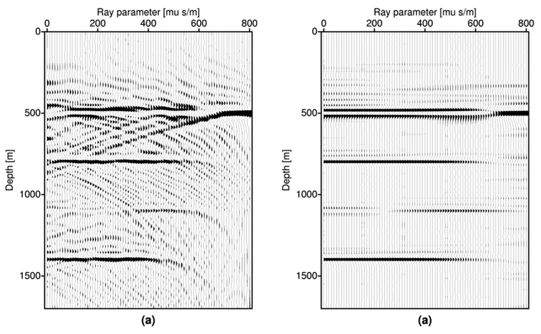
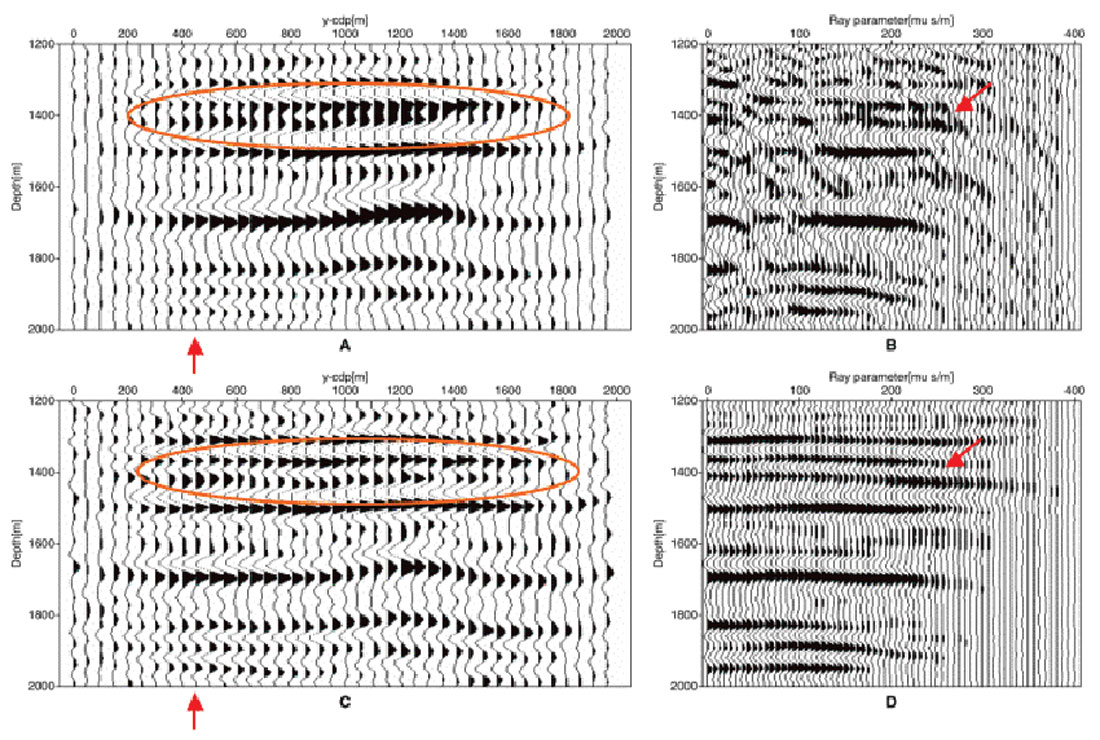
Figure 6 portrays a comparison of migration and regularized migration with quadratic regularization for a 3-D survey in the Western Canadian Sedimentary Basin (a complete description of the data and calibration of amplitudes with synthetics produced with sonic and density logs is provided in Wang et al., 2005). Figures 6a and 6b show the wave-equation migrated inline image and a common image gather at the position marked with a red arrow. Figures 6c and 6d display the resulting images and common image gather computed with regularized migration (quadratic constraint). The image computed via regularized migration not only provides common image gather with enhanced lateral continuity but also an inline stack with a substantial resolution enhancement (see the areas highlighted with the red ovals).

At this stage, our migration schemes are able to operate with quadratic regularization strategies that can provide an important enhancement of the lateral continuity of inverted common image gathers. Can we incorporate non-quadratic regularization terms into our seismic imaging framework? At present time, imaging via inversion with quadratic regularization is feasible; there exists algorithms that have been used with success to process small 3-D real data surveys (Wang et. al, 2005). These tools have not been incorporated into industrial production streams yet. We anticipate, however, that regularized migration/inversion methods do have a promising future in seismic data processing and imaging. In particular, the aforementioned methods can play an important role in the identification of thin layers and subtle stratigraphic targets; a problem often encountered in the exploration and development of new and existing plays in the Western Canadian Sedimentary Basin.

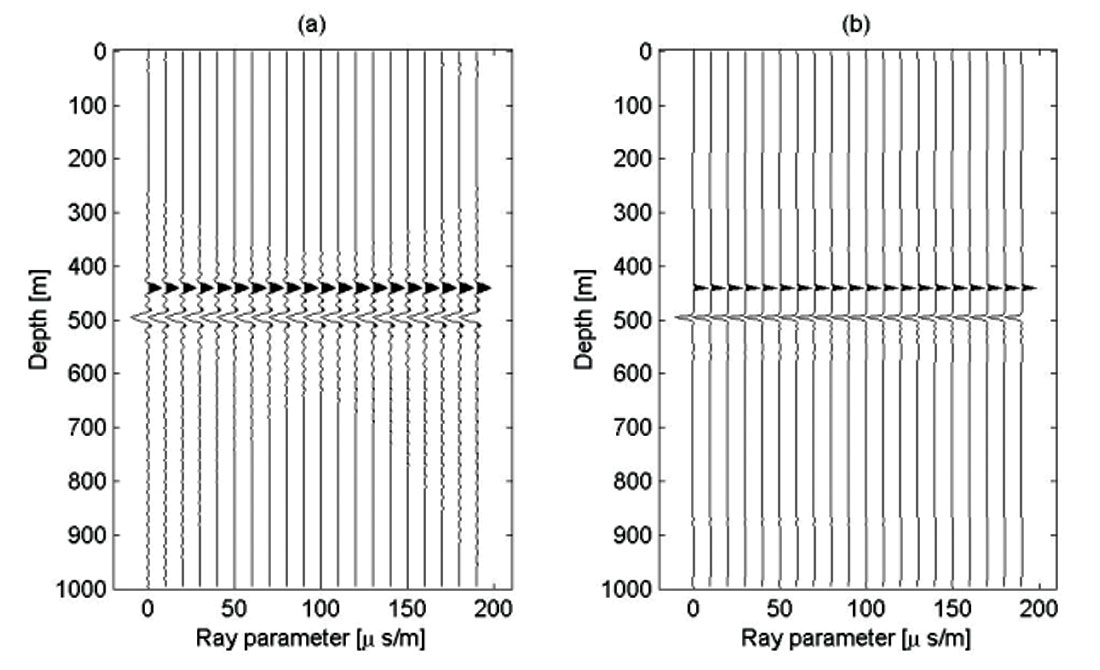
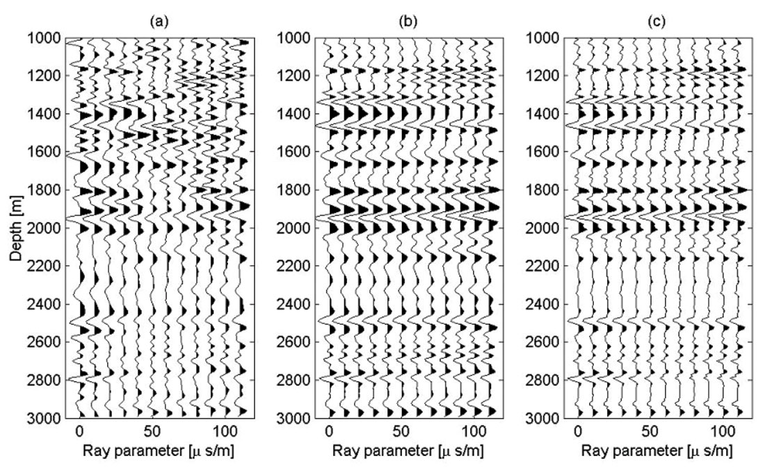
The incorporation of non-quadratic regularization terms into the inversion of common image gathers has been outlined by Sacchi et al. (2003) and tested with encouraging results by Wang and Sacchi (2005). So far, we have obtained encouraging results with inversion strategies with smoothing constraints in the horizontal ray parameter axis and sparseness in the vertical direction (depth). The latter is achieved via a Cauchy regularization term that not only enforces sparseness in depth but also preserves continuity along offset or ray parameter. This approach offers a bridge between well-known sparse-spike inversion methods for impedance recovery (based on the convolutional model) and migration / inversion methods. Our synthetic example in Figure 7 provides a comparison of regularized migration with ray parameter smoothing versus non-quadratic regularization with ray parameter smoothing plus sparseness in the vertical direction. The common image gather portrayed in Figure 7 corresponds to a 3-D synthetic were we have chosen a flat AVO response. The optimization procedure utilized to obtain sparse common image gathers is discussed in Wang (2005). Figure 8 portrays a real data comparison of migration, regularized migration with a quadratic constraint, and regularized migration with sparseness (non-quadratic regularization). These results correspond to a common image gather of the data set utilized in Figure 6 (3-D survey, Western Canadian Sedimentary Basin). It is interesting to point out that the wavelet ringing in Figure 6c is minimized because of the addition of a sparseness constraint.

High-resolution common image gathers in offset or ray parameter domain can be used for the subsequent inversion of petrophysical parameters and/or hydrocarbon indicators via standard AVO fitting methods. Regularized migration enables us to push the resolution limit that quite often hampers our ability for proper AVO processing. For instance, by extending the bandwidth of the inverted common image gathers, wavelet tuning can be attenuated.

Conclusions and Future Perspective on Regularized Imaging

Imaging/inversion with the introduction of quadratic and non-quadratic constraints could lead to a new class of imaging algorithms where the resolution of the inverted image can be enhanced beyond the limits imposed by the data (band-width and aperture). This is not a completely new idea. Geophysicists have been using similar concepts to invert post-stack data (sparse spike inversion) in an attempt to construct highly resolved impedance profiles. What constitutes an optimal regularization strategy for imaging problems is a topic of current study. At the present time, smoothing along the angular variable of the common image gathers (offset or ray parameter) plus vertical sparseness appears to be a regularization goal that is simple and consistent with the estimation of high resolution common image gathers for subsequent studies.

Future research directions call for methods to mitigate operator mismatch, efficient numerical optimization methods for large-scale problems, regularization methods capable of incorporating the reflectivity character (color) into our subsurface estimates and, extensive field data tests to properly assess the benefits of regularized migration.

Acknowledgements

We would like to acknowledge financial support and stimulating discussions offered by the industrial members of the Signal Analysis and Imaging Group. We thank Dr Scott Cheadle (Veritas DGC) for providing the field data used in this study. Support from the Natural Sciences and Engineering Research Council of Canada is also acknowledged.