Reflections on the Deconvolution of Land Seismic Data

Convolution is the process by which a wavelet combines with a series of reflection events to produce the seismogram that is recorded in a seismic survey. The familiar model is that a seismogram, s(t), is the wavelet, w(t), convolved with the reflectivity, r(t), and noise, n(t): s(t) = w(t) * r(t) + n(t). Deconvolution is the inverse process that removes the effect of the wavelet from the seismogram. Deconvolution attempts to compress the wavelet, thereby increasing the resolution of the seismic data. Another goal of deconvolution is to produce a wavelet with a simple phase character, ideally a zero-phase wavelet, which is the same for every trace in the seismic dataset.

Deconvolution is a topic that has received a lot of attention from geophysical researchers in previous decades, but these days it does not receive much attention compared to topics like migration, anisotropy and time-lapse imaging. Nevertheless, deconvolution continues to be a vitally important part of seismic processing, and as the reservoir targets that we explore and develop become more and more subtle, the need for correct and successful deconvolution becomes more and more important.

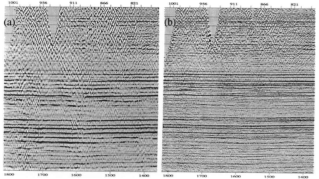
An example of why we apply deconvolution is shown by the difference between the two seismic sections in Figure 1. Note that the reflections in the dataset with wavelet processing are sharper and more compressed than without wavelet processing, which indicates that the frequency bandwidth has been improved. Also note that the reflections are more regular and continuous across the seismic section after wavelet processing so the deconvolution appears to have produced the desired similarity in the phase character from trace to trace.

The primary contribution to the wavelet that is embedded in a raw seismic trace is usually the source signature, but there are also contributions from many other parts of the raypath from source to receiver, such as the near-surface structure around the source and the receiver, source and receiver-side ghosts, the response of the receiver, the response of the recording system and the effect of attenuation along the raypaths. Ideally we would like to remove the effect of all of these contributions to the seismic trace before interpretation. The interpreter needs to be able to believe that a change to a reflector in the final seismic image is due to a change in the geology and is not due to some residual near-surface effect on the wavelet that deconvolution has not properly removed.

There are two general types of deconvolution, one where the wavelet is known or measured, which is called deterministic deconvolution, and the other where the wavelet is not known, which is called statistical deconvolution. It has become more common in the acquisition of marine seismic surveys to record the signature of the pressure pulse, which often is not minimum phase, in order to allow a signature deconvolution to convert the wavelet into a desirable shape.

In a recent article, Bill Dragoset (2005) states that:

From the 1970s through the 1990s, both kinds of deconvolution were routine data processing steps. More recently, the statistical approach has lost favour with many geophysicists who mistrust its reliance on assumptions that may not always be true.

It is obvious to anyone who works with land seismic data that Dragoset must be referring in this statement to the deconvolution of marine data because no move away from statistical deconvolution has occurred with the processing of land data. With land data we are still stuck with statistical deconvolution, and that shows no sign of changing anytime soon.

Although there has been some effort directed toward the recording of land source wavelets, no method has proven to be of practical use. It is not clear how useful such a measurement would be in any case. In the land situation the effect of the highly inhomogeneous near-surface layers immediately around the seismic source on the initial downgoing wavefield can be so complicated that it is unclear what measurement could be made in order to entirely capture the source plus near-source effects which together we want to deconvolve. And of course any measurement of the source wavelet would not include the receiver response, the receiver coupling effects and the near-surface effects around the receiver which we also want to deconvolve.

We do not know a priori what the wavelet is in the land situation, but we still need to come up with some estimate of it if we are to proceed at all. The statistical approach to deconvolution enables us to proceed. The price that we pay for using a statistical approach to deconvolution is that we are forced to accept its assumptions. Two important assumptions of statistical deconvolution are that the wavelet is minimum phase and that the reflectivity is white. These two assumptions together allow us to construct an estimate of the wavelet. The reflectivity assumption enables us to identify the power spectrum within the deconvolution design gate with the wavelet’s power spectrum. The minimum phase assumption allows us to construct the wavelet’s phase spectrum from its power spectrum.

Common seismic sources for land data acquisition are dynamite, Vibroseis and various kinds of weight-drop. Impulsive sources such as dynamite and weight-drop are assumed to be minimum phase in character and there is little concern about that assumption being incorrect. On the other hand, the accepted wisdom is that Vibroseis is a zero-phase source, so it needs to be converted to minimum phase as part of the deconvolution process. There has been doubt for a long time about the exact post-correlation pulse radiated by Vibroseis and its variation from place to place (White, 1987). Some very interesting observations by Dong, Margrave and Mewhort (2004) call the phase properties of the Vibroseis source into question and imply that the minimum-phase conversion of Vibroseis data is not what we should be doing.

The appropriateness of the assumption that the reflectivity is white is difficult to assess. We know from the study by Walden and Hosken (1985) that reflectivity functions are usually more blue than white, but deconvolving a seismogram with a blue reflectivity as if it is white does not have a harmful effect on the deconvolution results, as least visually. More of a concern, especially in areas where the sedimentary basin is relatively thin, is that the seismograms are not long enough to allow a statistically accurate measure of frequency content, or that a small number of closely-spaced strong reflectors within the design gate would introduce significant departures from whiteness. There are few known remedies in these situations. Often the most that can be hoped for is that the processor or the interpreter, or both, are aware of the dangers.

In addition to the minimum phase and reflectivity assumptions, statistical deconvolution assumes that the effect of noise is minimal, or at least that it is random and is uncorrelated with itself and with the signal. For land data this is usually too much to expect so a number of comments about the effects of noise need to be made.

A major contribution to any seismic trace that is acquired on land is noise. In the convolution equation noise is modeled as an additive effect but this model is clearly inadequate a lot of the time. For example, ground roll does not fit this expectation since it is generated by, and correlated with, the source. Noise is not something that we explicitly want to remove by the process of deconvolution since it is not part of the embedded seismic wavelet. However, noise plays an important role in determining the complete wavelet processing flow that is applied to land seismic data.

For example, suppose that powerline noise is present in the recorded data so that there are spikes in the amplitude spectra of the traces at 60 Hz and harmonics of this frequency. This is an effect that may appear to be embedded in the seismic wavelets since a spike likely occurs on many of the amplitude spectra of the seismic traces. Power-line noise is likely a surface-consistent effect as well. However, it is not something that we want deconvolution to remove because the seismic waves that propagate through the earth do not really contain spikes at those particular frequencies. The powerline noise would be measured before and after the seismic source is fired. We therefore want a separate process to remove the effects of powerline noise before deconvolution is performed. Fortunately, algorithms exist that can do a very effective job of removing powerline noise while leaving the signal spectrum intact. This is not true with many other types of noise.

In general, we would like to take the approach of removing all noise, especially coherent noise, from the seismic traces before performing deconvolution. Unfortunately, this is usually too much to ask because of our inability to separate signal from noise in a completely reliable manner. Although methods such as F-K filtering or other types of multichannel filtering are often used to remove source-generated noise before deconvolution, it is more common to use an appropriate combination of surface-consistent deconvolution, spectral whitening and CDP stack in order to reduce the impact of source-generated noise.

Surface-consistent deconvolution offers a relatively simple way to side-step some of the major influences of noise on deconvolution filters. The surface-consistent model assumes that there is one wavelet that is common to each source and receiver surface position within the total dataset. This assumption enables a significant amount of averaging to occur during the solution since it reduces the total number of unknowns to be resolved. By reducing the total number of wavelets that need to be resolved, surface-consistent deconvolution removes a lot of the noise-induced trace-to-trace fluctuations in the wavelet estimates that occur with trace-by-trace applications of deconvolution.

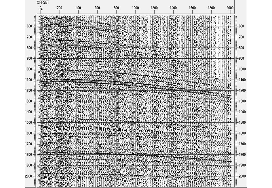
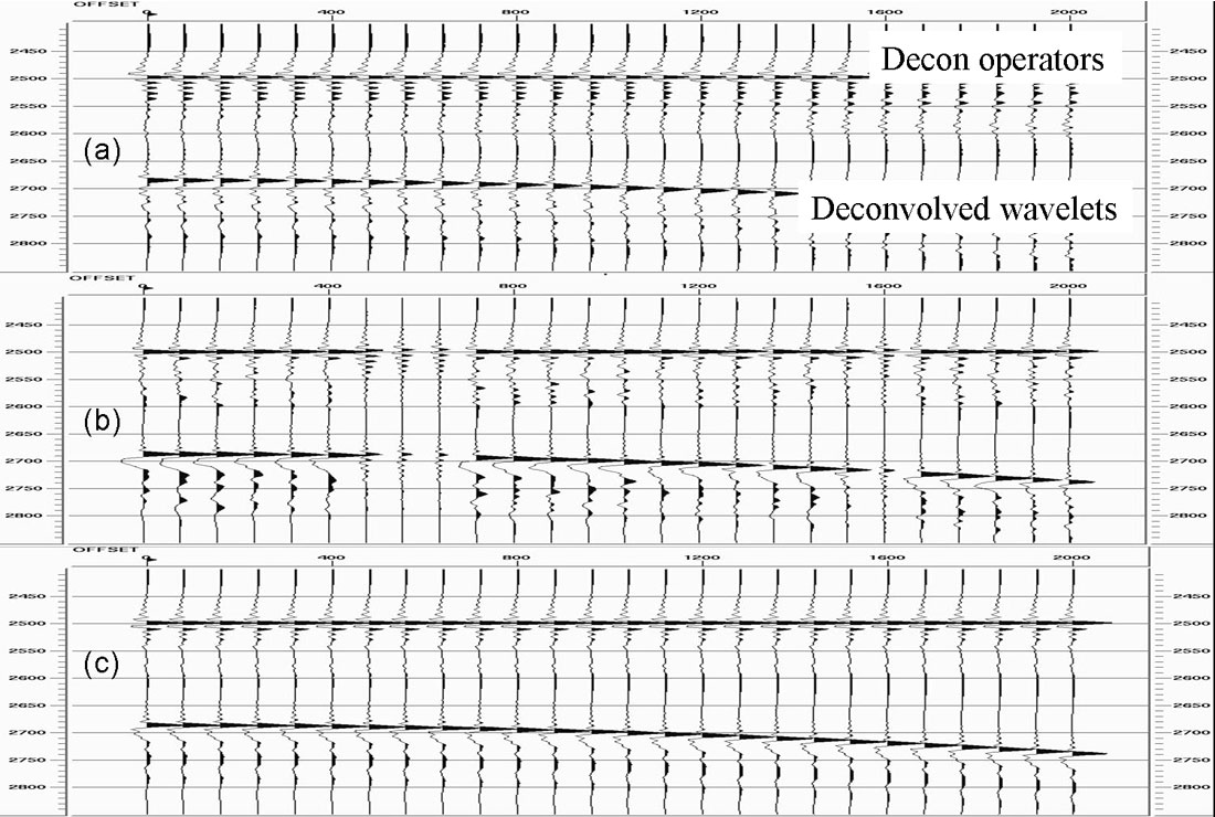
To illustrate the advantages of surface-consistent deconvolution over trace-by-trace deconvolution we can use a synthetic record. Figure 2 shows a synthetic source gather that has been generated by convolving a known minimum phase wavelet with a reflectivity series and adding random noise. The level of noise varies randomly from trace to trace, which is typical of real seismic records. Figure 3(a) shows the virtually perfect zero-phase result of trace-by-trace deconvolution when there is no additive noise. Figure 3(b) shows the highly-variable deconvolution operators and deconvolved wavelets that are the result of trace-by-trace deconvolution with the additive noise. Figure 3(c) shows the deconvolution operators and deconvolved wavelets that are the result of shot-consistent deconvolution, which is the best approximation to surface-consistent deconvolution that we can perform with this dataset with only one shot gather. Although the surface-consistent deconvolution result produces wavelets that are not zero phase, they can be rotated to a wavelet that is close to zero-phase with a single operator, which is the way that interpreters standardly match seismic sections to synthetic seismograms before interpretation. No single phase rotation operator could correct the trace-by-trace deconvolved wavelets in Figure 3(b). The consistently wrong result of surface-consistent deconvolution is therefore better than the inconsistently wrong result of trace-by-trace deconvolution.

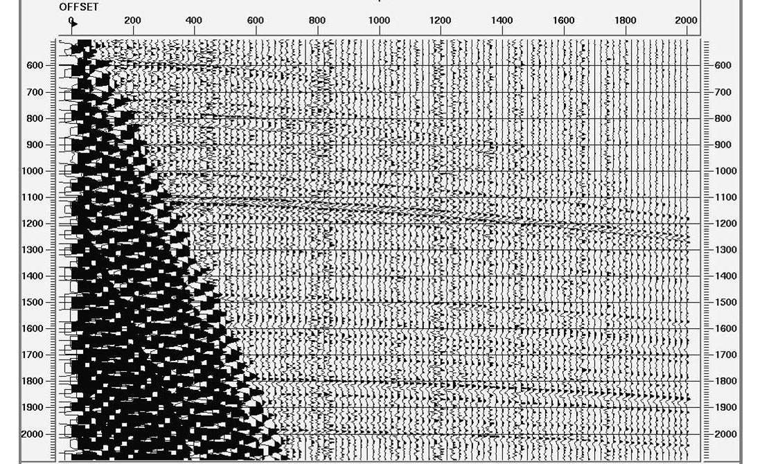
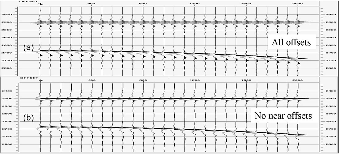
With surface-consistent deconvolution, it is also possible to use a deconvolution design gate that excludes the low-frequency, source- generated noise that contaminates the near-offset traces. This can be extremely important for stabilizing the phase of the output because the impact of low-frequency noise is primarily to cause an error in the phase of the final result (Berkhout, 1977). The amount of phase error would fluctuate with the level of noise, so it is wise to exclude the near offsets from the deconvolution design. Figure 4 shows the same gather as Figure 2, but with synthetic ground roll noise included at the near offsets. Figure 5(a) shows the results of shot-consistent deconvolution with a design gate that includes traces at all offsets. Figure 5(b) shows the comparable result with a design gate that excludes the ground roll. Notice that Figure 5(b) is essentially identical to Figure 3(c).

Much has been made at times of the potential advantages of the multiple components that can be included in the solution phase of surface-consistent deconvolution, but many of the advantages have been over-emphasized. There is some advantage to including an offset component in the surface-consistent solution as long as it is not included in the application phase, but there is little need for more components than source, receiver and offset. The advantages of surface-consistent deconvolution for reducing the impact of noise on the final results are obvious, so is easy to understand why it became widely used once an efficient algorithm was introduced (Cary and Lorentz, 1991).

Ideally, deconvolution filters should be designed on signal as much as possible, and not on noise. The implication, there f o re, is that deconvolution does not, and should not, perform noise attenuation. Nevertheless, there is a need for a full wavelet processing flow to attenuate noise to some degree in order to produce interpretable data. Spectral whitening, which is often applied in a time-variant form, is the most common way of attacking noise after surface-consistent deconvolution. It works by balancing the amplitude spectrum of each trace independently. If a trace contains a large amount of low-frequency noise, then the amplitude of those low frequencies is lowered to a level that is common with other frequencies within the bandwidth of the signal.

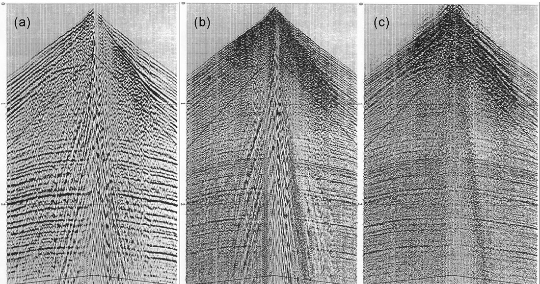
Figure 6 shows a real-data shot record (a) before deconvolution, (b) after surface-consistent deconvolution, and (c) after surface-consistent deconvolution plus time-variant spectral whitening. The surface-consistent deconvolution in Figure 5(b) has increased the frequency bandwidth of the data, but many reflectors are obscured by noise. The spectral whitening in Figure 6(c) has improved the signal-to-noise level of the data so that reflectors now appear much more continuous.

Spectral whitening is an extremely robust and effective noise attenuator, which explains why it is so widely used. However, there are two important notes of caution to be aware of with regard to spectral whitening. First, spectral whitening performs noise attenuation by forcing the level of noise down at certain frequencies, but it also forces the level of the signal down at those frequencies by the same amount. There f o re, the frequency content of the wavelets embedded in the data will be inconsistent after spectral whitening. Wavelets with inconsistent frequency content will have inconsistent amplitudes, so that spectral whitening is not something that should be performed before amplitude-versus-offset (AVO) analysis. Some other form of noise attenuation that does not significantly affect the signal should be applied if AVO is to be performed.

The second note of caution with respect to spectral whitening is that we should expect the wavelets after CDP stack to be deficient in certain frequencies because of the inconsistent frequency content of the prestack wavelets. So even with the application of perfect NMO-velocities, we should not be surprised to see that spectral whitening needs to be applied to the stacked data in order to restore the full frequency content of the signal that the prestack spectral whitening reduced. This at least partly explains why the widely-used poststack application of spectral whitening and f-x deconvolution is so effective at increasing the bandwidth of the final stacked seismic data.

Besides performing noise attenuation, time-variant spectral whitening also attempts to remove the time-dependent loss of high frequencies in the data due to attenuation, while leaving the phase of the data the same. An alternative method for reversing the effects of Q is to explicitly apply an inverse Q-filter before deconvolution. Although practical methods for inverse Q-filtering have existed for many years (e.g. Hargreaves and Calvert, 1991; Hale, 1982), inverse Q-filtering has never become a standard element of the seismic processing flow. Perhaps this is because the time-dependent phase correction that it entails has never been seen to be very important. For most interpretation, all that really matters is that the wavelet phase is correct at the zone of interest, and this can be accomplished without inverse Q filtering. Gabor deconvolution (Margrave et al., 2003) is a recent attempt to incorporate data-adaptive inverse Q-filtering with a trace-by-trace deconvolution algorithm.

This review of the present state of deconvolution has mostly focused on the impact of the various assumptions that are built in the standard wavelet processing flows of land data. The various types of noise that are present in land data have an important influence on the wavelet processing flow. At the present time, we do a relatively good job of whitening the amplitude spectrum of the signal in our data. However, there is a lack of control over the phase of our data after deconvolution. This is not considered to be a problem by most interpreters as long as the phase can be rotated back to zero with a constant rotation operator. There is definitely a problem, however, if the phase varies laterally along a seismic line. There is no absolute guarantee with our present methods of processing data to ensure complete phase stability after deconvolution, so this is an area of research that deserves attention in the future.