Reflections on Q

Abstract

Seismic reflections are generally caused by contrasts in acoustical impedance. However, in media where there is significant absorption of seismic energy, reflections can also be caused by contrasts in the seismic absorption coefficient (or inverse-Q values). This note derives the reflection coefficient for a normally incident acoustical wave and then uses seismic modeling of SH-wave reflections for absorptive media using the finite-difference codes of Carcione (2007). Both theory and modeling predict that seismic absorption contrasts create weak reflections that are phase shifted from reflections caused by impedance contrast alone.

Introduction

Exploration seismologists normally consider seismic reflections to be caused by contrasts in acoustical impedance (product of seismic velocity and density). However, in media where there is significant absorption of seismic energy, we can have reflections that are caused by contrasts in the seismic absorption coefficient, α . Contrasts in absorption can also be considered as contrasts in the quality factor, which is inversely proportional to absorption.

This paper considers the model response and mathematical derivation of reflection coefficients for SH-waves. The SH-wave reflection case is simple in that it involves no mode conversions. However, the case is relevant to exploration seismology, since as pointed out by Shearer (1999), the reflection coefficients and boundary conditions for normally indident SH-waves for a layered medium have the same mathematical form as normally incident P-waves. In the case of SH-waves, the boundary conditions require continuity of horizontal displacement and traction, while in the case of P-waves, the boundary conditions require continuity of normal displacement and normal stress. Derivations for SH-waves (Shearer, 1999) and P-waves (Robinson and Treitel, 1980) produce the same form of reflection coefficients.

For modeling SH-wave reflections in absorptive media, the finite-difference codes found in Carcione (2007) prove to be very useful. We now consider some modeling examples. Figure 1 shows a two-layer model of 1200 m by 1200 m, with 120 x 120 grid points with grid spacing of 10 m. The boundary between the layers is at a depth of 400 m. A source is placed at a depth of 250 m, at the horizontal midpoint, x=600 m. In order to avoid ghosting in the model, receivers were placed at a depth of 260 m with horizontal spacing of 10m across the model. The layers all have constant density (2.2 gm/cc).

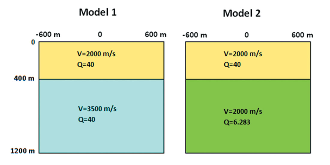
In initial tests, synthetic seismograms were computed with the following parameters:

1. Test 1, layer 1 velocity = 2000 m/s, layer 2 velocity=3500m/s, Q=40 for both layers 1 and 2.
2. Test 2, layer 1 velocity=2000 m/s, layer 2 velocity=2000m/s, Q=40 for layer 1, Q=6.283 for layer 2.

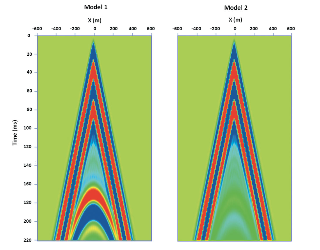
Figure 2 shows two reflection seismograms for SH mode propagation obtained using seismic modeling codes by Carcione (2007). In Figure 2 (left), the reflections are caused only by a contrast in acoustical impedance in a two-layer model where the velocity increases from 2000 m/s to 3500 m/s. In Figure 2 (right), there is no impedance contrast but there is a contrast in Q from Q=40 to Q=6.283. We see reflections that are not as strong for the second case, but reflections occur nonetheless. Hence, it would appear that reflections in the second seismogram are due solely to contrasts in the absorption, which is related to the quality factor, Q, by the relationship:

Here

is the wavelength, ν is the seismic velocity and f is the temporal frequency of the wave.

Methodology and results

To show how these reflections arise from absorption contrasts, we extend the reflection coefficient derivation given by Robinson and Treitel (1980, p. 296) to allow for absorption. The original Robinson and Treitel boundary conditions were computed for normally incident P-waves, whereas our numerical computations with Carcione’s codes were for SH waves, that undergo no mode conversions. At normal incidence, these are essentially the same type of boundary conditions.

Following the notation of Robinson and Treitel (1980), we consider a layer boundary at y=0 where y, the depth dimension is increasing downward. The incident, reflected and transmitted sinusoidal wave displacements are given by:

and

For an elastic medium, the wavenumbers κ₁,κ₂ are real and given by:

and

where ν₁, ν₂ represent the seismic velocities in layers 1 and 2. These wavenumbers are real for a medium that is purely elastic with no energy loss to absorption, which is the case where α = 0.

However, we can readily consider absorption by introducing a wavenumber that is complex and given by:

or alternatively,

Toksoz and Johnston (1980), among others, explain this concept of a complex wavenumber whose imaginary component is absorption.

To derive the displacement reflection coefficients for this absorptive medium for a normally incident plane wave, we follow Robinson and Treitel’s method (1980) and require that the displacement and the normal stress be continuous at a boundary. The continuity of displacement at y=0 requires that:

(Here we divided out a common exponential factor, exp(2πift) .)

The continuity of normal stress requires that

be continuous where Ε is the elastic constant relating stress to strain. Therefore,

If we replace Κ by κ in the displacement expressions of (2), (3) and (4) and substitute these into equation (10), after dividing out a common factor of exp (2πift) we obtain the following boundary condition at y=0:

Now if we combine equation (9) with equation (11), we obtain the expression for the reflection coefficient:

We can express Εκ in terms of density, ρ , and velocity, ν while recalling that E = ρν² . Therefore Εκ can be expressed as:

If we express equation (13) in terms of Q, we get

which can be rewritten as:

Equation (15) is consistent with the complex wavenumber resulting from Aki and Richards (1980, p. 182). If we substitute equation (15) into equation (12), we obtain the following expression for the reflection coefficient in absorptive media, after dividing numerator and denominator by 2πf :

If there is no absorption in the medium (infinite Q) such that the

terms vanish, equation (16) reduces to the difference of acoustical impedances divided by the sum as given by Robinson and Treitel (1980). On the other hand, if there is no acoustical impedance contrast between medium 1 and medium 2, we can still obtain reflections due to a contrast in absorption (inverse Q). In such a case, the reflection coefficient is given by:

Therefore, even with no impedance contrast, we can have reflections due to a contrast in the absorption properties of two layers.

Given the nature of finite Q in absorptive media, there is an important characteristic of R in equations (16) and (17) that is different from the non-absorptive case. Futterman (1962) shows that absorption is linked to wave dispersion through a Hilbert transform relationship, and that Q necessarily has a frequency dependence for absorptive media. Therefore, the reflection coefficient, as expressed in (16) also has a frequency dependence.

In Figure 2, we show the results of some finite-difference calculations for SH-waves for two cases: where the impedance contrast is 2:3.5, and where the Q contrast is 40:6.283. The reflection coefficient for the first case (where Q is constant) would simply be equation (16) with the Q and density contributions cancelling out leaving the difference in velocity divided the sum of the velocities,

The reflection coefficient for the second case (with no impedance contrast) would be obtained by substituting into equation (17) to give:

or

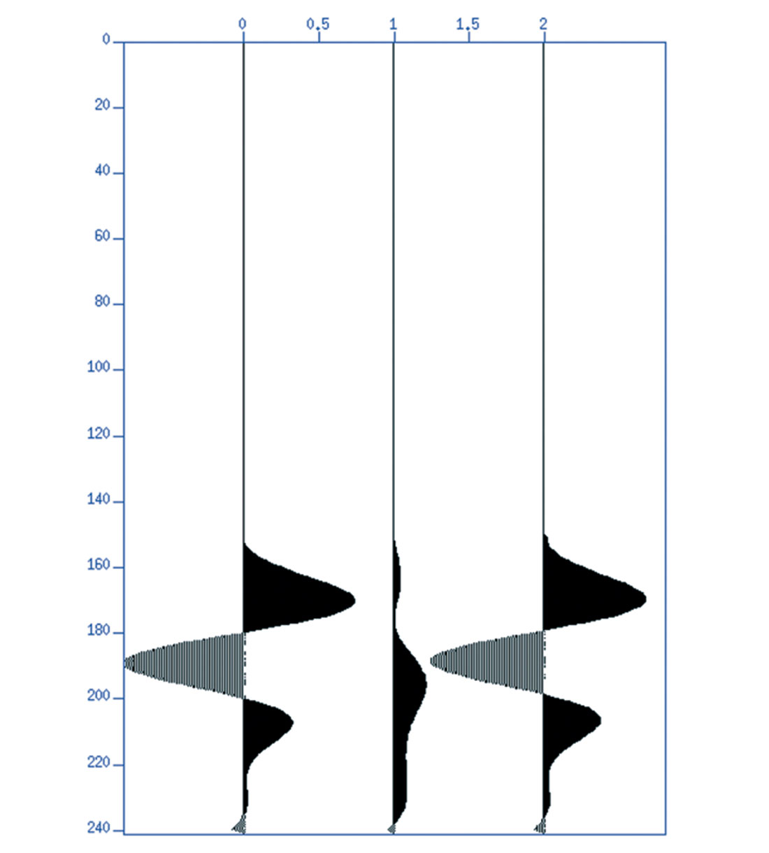
This is a complex number whose amplitude is about 1/8 as big as the reflection coefficient for the impedance contrast, and there is a phase shift due to absorption. If we include both an impedance contrast and a Q contrast, the resulting seismic trace is not significantly different from that of the impedance contrast only. Figure 3 shows the normal incidence traces of the seismograms for impedance contrast only (leftmost trace), Q contrast only (middle trace) and for impedance contrast and Q contrast. The reflection amplitude for the left trace is nearly identical to the right trace. Although the absorption contrast reflection is nonzero and phase shifted from the impedance reflection, this difference is barely noticeable.

Conclusions

Using both theory and numerical modeling we have shown that the inclusion of absorption in our reflection computations, both in boundary value analysis and finite-difference calculations, produce reflection amplitudes that are slightly phase shifted but not noticeably different from those derived from elastic reflection coefficient calculations. While the reflections from Q contrasts are scientifically interesting, they are unlikely to be of significant importance in realistic geological situations.

Acknowledgements

We thank the sponsors of this research including the Consortium for Research in Elastic Wave Exploration Seismology (CREWES), Consortium for Heavy Oil Research by University Scientists (CHORUS) and the Natural Sciences and Engineering Research Council of Canada (NSERC). We thank the late Dr. Kit Crowe, formerly of Amoco Research, for providing unpublished discussions on the concepts of Q reflections. Finally, we are grateful to Dr. Enders Robinson and two anonymous reviewers for their constructive and helpful review of this paper.