Recent Advances in Rock Physics and Fluid Substitution

Understanding the Rock Physics Links Between Geologic Processes and Seismic Signatures

One of the most important developments in rock physics has been progress toward quantifying the relations between geologic processes and geophysical signatures. Historically, the majority of rock physics research was done by physicists. Their theoretical models – some very useful – described the effective properties of the rock as a mechanical system of mineral grains, pores, and pore fluids. From theory and observation, we learned that details of the rock microtexture – pore shapes, pore connectivity, grain size and shape distributions, the nature of grain-to-train contacts, and variations in mineralogy – are important for understanding rock’s porosity, permeability, electrical, and elastic properties. Finally, during the last decade, a significant effort in rock physics research has refocused on understanding the relations between rock properties and the depositional and diagenetic processes, which create and control the rock texture.

The Elastic Bounds

Effective medium models for the elastic properties of rocks generally require three types of inputs: (1) the volume fractions of the rock and fluid constituents, (2) the elastic moduli of the various phases, and (3) the geometric details of how the phases are arranged relative to each other. Of these, the geometric details have never been adequately incorporated into models.

When we specify only the volume fractions of the constituents and their elastic moduli, without geometric details of their arrangement, then we can only predict the upper and lower bounds on the moduli and velocities of the composite rock. The simplest bounds are those by Voigt (1910) and Reuss (1929). The Voigt upper bound on the effective elastic modulus, M_V of a mixture of N materials phases is (Voigt, 1910)

where f_i is the volume fraction of the ith constituent, and M_i is the elastic modulus of the ith constituent. The Reuss lower bound of the effective elastic modulus, M_R, is (Reuss, 1929)

There is no way that nature can put together a mixture of constituents and have it be elastically stiffer than the linear average given by the Voigt bound or softer than the harmonic average of moduli given by the Reuss bound. The best bounds for an isotropic elastic mixture, defined as giving the narrowest possible range of elastic moduli without specifying anything about the geometries of the constituents, are the Hashin-Shtrikman bounds (Hashin and Shtrikman, 1963; Berryman, 1995).

The Bounds as Models for Depositional and Diagenetic Trends

The elastic bounds provide a useful framework for understanding elastic properties of sediments. Figure 1 shows P-velocity vs. porosity for a variety of water-saturated sediments, ranging from ocean bottom suspensions to consolidated sandstones. The Voigt and Reuss bounds for mixtures of quartz and water are shown for comparison.

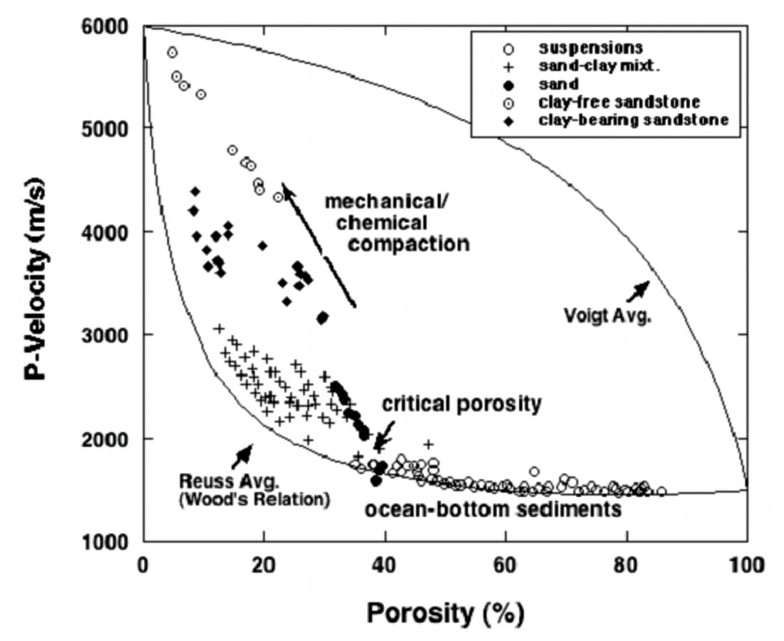
Before deposition, sediments exist as particles suspended in water (or air). As such, their acoustic properties must fall on the Reuss average of mineral and fluid. When the sediments are first deposited on the water bottom, we expect their properties to still lie on (or near) the Reuss average, as long as they are weak and unconsolidated. Their porosity at deposition is determined by the geometry of the particle packing. Clean, well-sorted sands will be deposited with porosities near 40%. Poorly sorted sands will be deposited along the Reuss average at lower porosities. Chalks will be deposited at high initial porosities, 55-65%. We sometimes call this porosity of the newly deposited sediment the critical porosity (Nur, 1992). Upon burial, various processes give the sediment strength – effective stress, compaction, and cementing – and move the sediments off of the Reuss bound. We observe that with increasing diagenesis (mechanical and chemical compaction), the rock properties fall along steep trajectories that extend upward from the Reuss bound at critical porosity, toward the mineral end point at zero porosity.

The bounds are useful for describing diagenetic and depositional trends as illustrated schematically in Figures 2 and 3. Diagenetic trends, which connect the newly-deposited sediment on the Reuss bound with the mineral point, can often be described using a modified upper bound, so-named, because we use it to describe a mixture of the newly deposited sediment at critical porosity with additional mineral, instead of describing a mixture of mineral and pore fluid. The modified upper Hashin-Shtrikman bound approximating the diagenetic trend for clean sands is shown by the heavy black curve in Figure 2. The dashed black curves below (and parallel to) the clean sand line represent the diagenetic trends for more clay-rich sands. They are computed again using the Hashin-Shtrikman upper bound, connecting the lower critical porosities for more clay-rich sands with the elastically softer mineral moduli for quartz-clay mixtures.

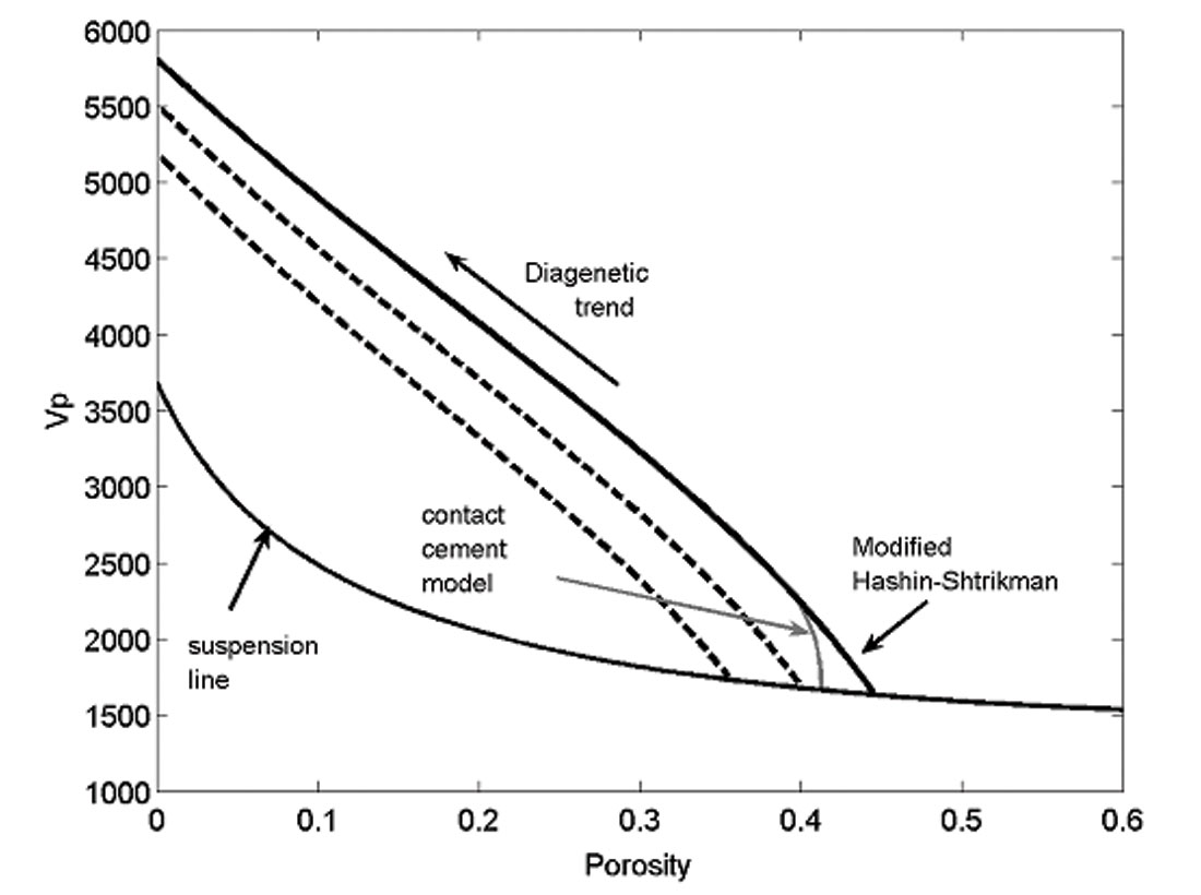
Slight improvement over the modified upper Hashin-Shtrikman bound as a diagenetic trend for sands is obtained by steepening the high porosity end. An effective way to do this is to append Dvorkin’s model (Dvorkin and Nur, 1996) for cementing of grain contacts (gray line, Figure 1). The contact cement model captures the rapid increase in elastic stiffness of sand, without much change in porosity as the first bit of cement is added. Florez (personal communication, 2003) has shown that very different processes such as mechanical compaction and pressure solution can yield very similar trends.

Depositional or sorting trends can be described with a series of modified Hashin-Shtrikman lower bounds (gray curves in Figure 3). The lowest gray curve is the suspension line, indicating depth = 0 (i.e., at the depositional surface). The additional gray curves above the suspension line indicate diagenetically older sediments. Each is a line of constant depth, but variable texture, sorting, and/or clay content. (Avseth et al., 2001, also refer to these as constant cement lines.) Moving to the right on the gray sorting curves corresponds to cleaner, better sorted sands, while moving to the left corresponds to more clay rich or more poorly sorted sands.

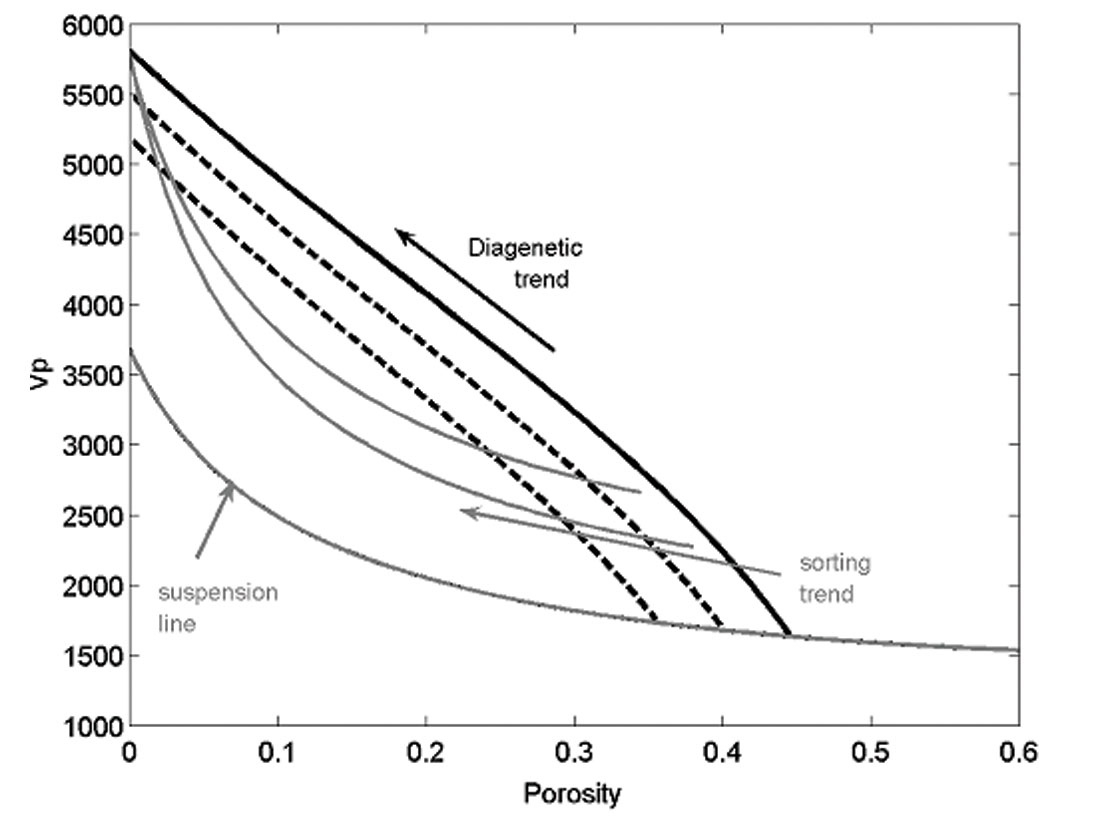
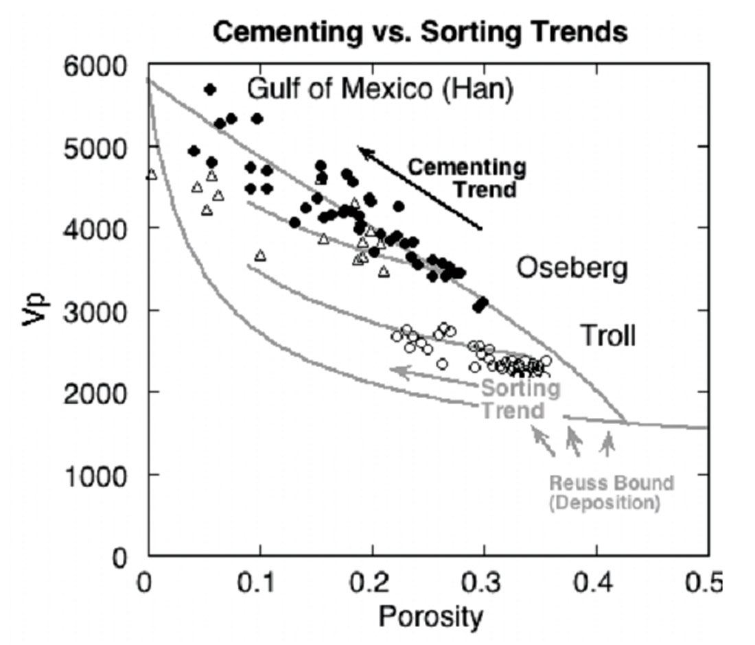
Figure 4 shows some laboratory data examples. The data from Han (1986), which span a great range of depths and ages, show the steepest average trend. Data from the Troll (Blangy, 1992), Oseberg, “N. Sea B”, and “N. Sea C” fields have flatter trends, dominated by sedimentation-controlled textural variations. The data from the “N. Sea A” field are from a narrow depth range, but in this case the porosity is diagenetically controlled, related to varying amounts of chlorite, giving a steep slope, close to Han’s.

A series of model refinements have been developed, specifically for high porosity clastics, each to be used for different geologic scenarios (for details, see Avseth et al., 2005):

• The friable (unconsolidated) sand model describes the velocity-porosity behavior versus sorting at a specific effective pressure. The velocity for the well-sorted, high porosity member (at critical porosity) is determined by contact theory, and intermediate (poorly sorted) porosities are “interpolated” using a lower bound.
• The contact cement model describes the velocity-porosity behavior versus cement volume at high porosities. The contact cement fills the crack-like spaces near the grain contacts. This cement tends to eliminate further sensitivity to effective pressure in the model. The high porosity member is the critical porosity, which can vary as a function of sorting. Poorly sorted cemented sandstones are then modeled using the constant cement model.
• The constant cement model describes the velocity-porosity behavior versus sorting at a specific cement volume, normally corresponding to a specific depth. The high porosity member is defined by first applying the contact cement model and calculating the velocity-porosity for a well-sorted sandstone with a given cement volume. A lower bound interpolation between this well-sorted end member and zero porosity will then describe more poorly sorted sandstones with the constant cement.
• The increasing cement model (modified Hashin-Shtrikman upper bound) describes the velocity-porosity behavior versus cement volume for low to intermediate porosities. The high-porosity end member is determined by contact theory. The first 2-3% cement should be modeled with the contact cement model. Further increase in cement volume and decrease in porosity is described by an upper bound interpolation between the high porosity end member and the mineral point.
• The constant clay model describes the velocity-porosity behavior for shales or sands with a constant clay-quartz ratio. The same equations are used as for the friable sand model. However, the high-porosity end member will vary as a function of clay content. The mineral end member is defined by effective mineral moduli of quartz and clay. A lower bound interpolates between the two end members.
• Dvorkin-Gutierrez shaly sand model describes the velocity-porosity relation versus clay content for shaly sands, assuming the clay is pore-filling. The high porosity end member is the same as for the friable sand model, while the low porosity end member is when the original sand porosity is completely filled with clay. However, this is not at zero porosity, since clay has intrinsic porosity.
• Dvorkin-Gutierrez sandy/silty shale model describes the velocity-porosity behavior versus clay content for sandy/silty shales. The high porosity end member is the pure shale, which can be calculated using the constant clay model with 100% clay. The low-porosity end member is the same as the low-porosity end member for the Dvorkin- Gutierrez sandy shale model.
• Yin-Marion shaly sand model explains the relationship between velocity-porosity-clay in unconsolidated sands. It assumes the clay to be a part of the pore-fluid, hence there is no increase in shear stiffness with increasing clay content for shaly sands. Gassmann theory is used to calculate velocity-porosity relations for increasing clay content.
• Yin-Marion silty shale model describes velocity-porosity behavior in shales with dispersed silt particles. The high porosity member is the pure shale, while increasing silt content will reduce this porosity. The low porosity end member will be when quartz grains start to touch each other, and the sediment becomes a shaly sand. Yin-Marion used Reuss (lower) bound to interpolate between these end members.
• Jizba’s cemented shaly sand model expands on the Yin- Marion model and takes into account quartz cementation. The quartz cement volume is estimated as a function of clay content. Empirical equations are used to calculate velocity-porosity relations as a function of quartz volume and clay content.
• The laminated sand-shale model calculates the effective velocity-porosity trends in thin-laminated sand-shales using the absolutely lower elastic bound, which is the Reuss bound.

Computational Rock Physics

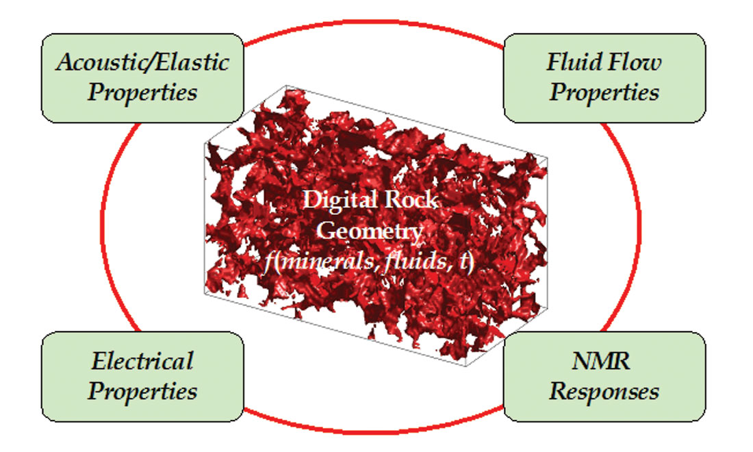
Scientific computing is one of the fastest developing branches of science and technology. The advent of cheap and powerful computers, as well as progress in computer architecture and parallel computing, make it possible to conduct extremely complex and realistic simulations of physical phenomena. Contemporary scientific computing allows scientists to conduct virtual (computational) experiments on digital representations of complex objects – in our case, rocks and sediments. Decades ago, before the availability of computational power, analytic models of rocks emerged using necessarily idealized pore geometries – ellipsoidal pores or spherical grains to model elastic properties, planar discontinuities to represent fractures, and tube networks to model permeability. While often yielding useful insights, these models were difficult to relate in detail to real rocks and sediments. Furthermore, it was virtually impossible to model the theoretical relations among such diverse properties as permeability, elastic moduli, electrical resistivity, NMR response, and failure strength. It was similarly difficult to model how this suite of properties would jointly evolve with variations in stress, diagenesis, chemical alteration, etc. However, more recently, combining computational advances with developments in rock physics theory has helped us to better attack problems related to the behavior of porous reservoir systems (e.g. Keehm et al., 2001). Now we can simulate multiple physical responses on models with realistic pore microstructure (Figure 5). We envision that computational rock physics will take the study of rocks to a new level, where reproducible experiments will be carried out on digital representations of the complex pore space.

Numerical experimentation cannot replace physical laboratory measurements. However, a computational environment can significantly complement the physical laboratory, with several distinct advantages:

• Simulations can be made that are faster and cheaper than some of the physical laboratory measurement counterparts.
• Interrelations among the different physical responses (e.g. permeability vs. NMR, dielectric vs. elastic, electrical conductivity vs. heat transfer) can be explored using a shared digital rock model. Such comparisons with corresponding physical laboratories are difficult, if not impossible, since measurements of different properties in a physical laboratory usually require different apparatuses and often, different samples.
• Physical responses of dynamic systems can be simulated – for example, how the transport or elastic properties of a medium evolve because of compaction, stress, or chemical changes.

Virtual experimentation can produce a new database stemming from a set of virtual and physically allowable variants of the original rock model, a goal that is essentially impossible to achieve in the real laboratory. Then experimentation becomes process-oriented and allows the scientist and student to understand how the porous medium and its physical properties evolve together with changing environmental conditions. Such quantitative understanding will not only produce a new database but can potentially lead to discovery of new scientific interrelations among various physical properties.

Statistical Rock Physics

One of the important current and emerging trends is the development of statistical rock physics techniques for reservoir characterization. By combining rock physics models with modern statistical techniques, together with seismic attributes, we can quantify uncertainties in interpretations of seismic attributes for reservoir exploration. In addition to quantifying uncertainties, the general framework is also useful for identifying additional information that may help to reduce the uncertainties. Rock physics allows us to establish the links between seismic response and reservoir properties. Monte Carlo simulations help to incorporate natural variability, and extend the available data to generate training data for statistical classification. Seismic imaging brings an indirect, but nevertheless spatially extensive, lateral and vertical information about the reservoir properties that are not available from well data alone. Classification and uncertainty estimation methods based on computational statistical techniques such as Bayesian classification, Monte Carlo simulation and bootstrap, help to quantitatively measure the interpretation uncertainty and the mis-classification risk. With geostatistical simulations, the spatial correlation and the small scale variability is added which is hard to identify with seismic information alone because of the limits of resolution. Combining deterministic physical models with statistical techniques helps us to develop new methods for interpretation and estimation of reservoir rock properties from seismic data. These formulations identify not only the most likely interpretation but also the uncertainty of the interpretation, and serve as a guide for quantitative decision analysis.

The statistical rock physics methodology may be broadly divided into the following steps: Briefly, first, the well log information is analyzed to obtain facies definition, after appropriate corrections, fluid substitution and shear velocity estimation when required. Basic rock physics relations such as velocity-porosity, and Vp-Vs are defined for the facies. This is followed by Monte Carlo simulation of seismic rock properties (Vp, Vs, density) and computation of the facies dependent statistical pdfs for various possible seismic attributes of interest (e.g. reflectivity, AVO gradient, near and far offset impedance, anisotropy parameters etc.) Monte Carlo rock physics modeling is used to extend the pdf’s to situations not encountered in the wells (e.g. different fluid saturations, presence of fractures). Following this, the seismic data (attributes) from seismic inversion or analyses (e.g. AVO analyses, impedance inversion, etc.) are used, in a statistical classification technique to classify all voxels within the seismic attribute cube.

Calibrating the attributes with the probability distributions defined at well locations allows us to obtain a measure of the probability of occurrence of each facies. Geostatistics is used to include the spatial correlation, represented by the variograms, and the small-scale variability, which is not captured in seismic data because of its limited resolution. Spatial variability can be incorporated at two stages: pre-inversion or post-classification. Early on during the inversion of seismic attributes geostatistical simulations can be used to build the models with the appropriate spatial correlation. Alternatively, after statistical classification of seismic attributes, spatial correlation can be incorporated by using the classification results as a soft indicator in a post-classification geostatistical simulation.

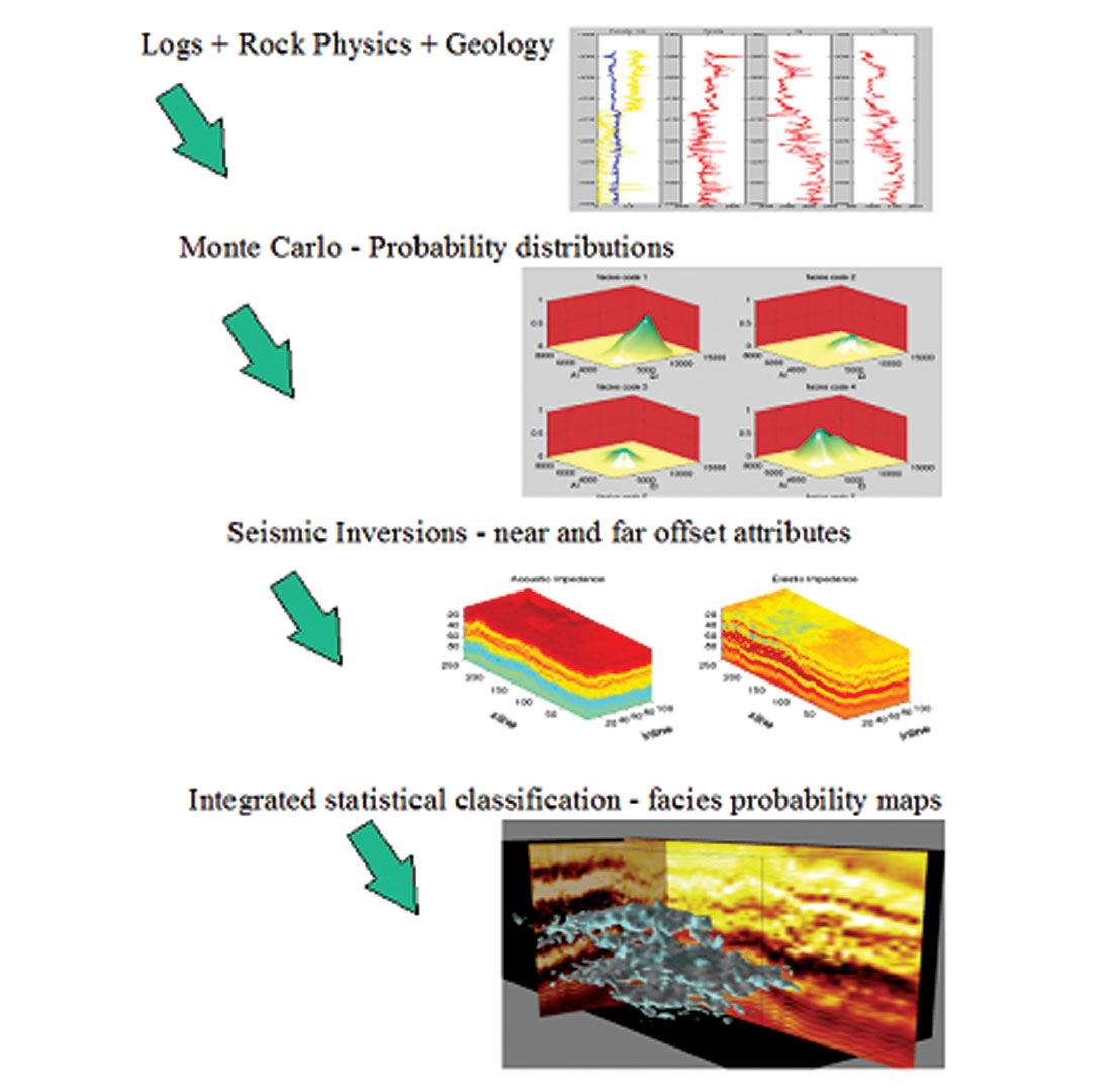
Pictorially, the steps are described in Figure 6: Well-log analysis, rock physics diagnostics, and facies definition; statistical rock physics, and estimation of facies-conditioned pdfs of seismic attributes from well log data; selection of attribute or attribute combinations based on information content for the targeted problem; estimation of attributes from seismic data using various inversion methods; Bayesian classification of the volumes of seismic attributes into different facies categories based on the facies conditioned, calibrated pdfs; and finally integrating spatial variability using geostatistics. The final products of this integrated technique are the spatial distribution of probabilities of reservoir fluids and facies, and stochastic realizations of the reservoir properties. In this way, not only do we obtain the most probable facies, but we can also quantify the uncertainty of the interpretation.

Statistical simulation has become a popular numerical method to tackle many probabilistic rock physics problems. One of the steps in many statistical simulation procedures is to draw samples X_i such that they follow a desired probability distribution function F(x). Once a large number of samples are drawn, the desired function is computed from the drawn samples. This procedure is often termed as Monte Carlo simulation, a term made popular by physicists working on the bomb during WWII. In general Monte Carlo simulation can be a very difficult problem, specially when X is multivariate with correlated components, and F(x) is a complicated function. One of the issues when using Monte Carlo simulation in rock physics, is to properly account for the correlations between the different rock properties. For example, simulations of Vs cannot be completely independent of simulated Vp and porosity values. Appropriate rock physics models and well log data should be used to do correlated Monte Carlo simulations. Complicated F(x) may require the use of iterative Monte Carlo methods such as Markov Chain Monte Carlo (McMC). Markov chain Monte Carlo is a sequential procedure that allows one to draw samples X_i using mathematical properties of Markov chains. Markov chain Monte Carlo is a powerful, numerically intensive procedure that has been applied in various fields of science and engineering to solve complicated probabilistic problems, and has begun to be applied in rock physics interpretation (e.g. Eidsvik et al., 2002).

Some of the future trends in applied statistical rock physics will include: strategies to better understand, quantify, and integrate qualitative, ‘fuzzy’ geologic information in terms of probabilities for seismic interpretation of reservoir properties; a better understanding of statistically combining different attributes such as attributes based on wave attenuation and mode conversion; integrating rock property variability with spatial uncertainty and geometric attributes, and emphasis on understanding uncertainties and risks associated with the geophysical interpretation, in order to incorporate them in to the decision making process.

When using statistical data-mining techniques it is wise to keep in mind some of the myths and pitfalls of these methods. It is a myth in that the more attributes we throw in, the more effective will be the statistical effort. More attributes are useful only if they can contribute more information about the goal of the exercise. Otherwise, they can do more harm than good. No statistical technique is so powerful that it can substitute for expertise in reservoir analysis and rock physics understanding of reservoir processes.

Fluid Substitution Analysis

At the heart of the fluid substitution problem are Gassmann’s (1951) relations, which predict how the rock bulk modulus changes with a change of pore fluids, with the companion result that the shear modulus is independent of the pore fluids. While Gassmann’s equations are quite general and robust, they nevertheless, were derived under several assumptions:

• The rock is monomineralic
• The pore space is very well connected
• The seismic frequency is low
• The saturating pore fluid is homogeneous

Most current research in fluid substitution analysis is aimed at learning how to apply the Gassmann relations to real rocks, which often violate these model assumptions. For example, the porosity, ϕ is normally interpreted as the total porosity, though in shaly sands the proper choice of porosity is not clear. We sometimes find a better fit to field observations when effective porosity is used instead. The uncertainty stems from Gassmann’s assumption that the rock is monomineralic, in which case the porosity is unambiguously all the space not occupied by mineral. Clay-rich sandstones actually violate the monomineralic assumption, so we end up forcing the Gassmann relations to apply by adapting the porosity and/or the effective mineral properties. Should the clay be considered part of the mineral frame? If so, does the bound water inside the clay communicate sufficiently with the other free pore fluids to satisfy Gassmann’s assumption of equilibrated pore-fluid pressure? – or should the bound water be considered part of the mineral frame? Alternatively, should the clay be considered part of the pore fluid? If so, then the functional Gassmann porosity is actually larger than the total porosity, but the pore fluid should be considered a muddy suspension containing clay particles. Extensions of the Gassmann equations to mixed mineralogies (Brown and Korringa, 1977) and anisotropy (Gassmann, 1951; Brown and Korringa, 1977) exist, though they require additional material constants, which are seldom known in the field. Current research is aimed at finding valid approximations that will allow fluid substitution analysis in the field, when only limited information about the anisotropy is available. Another area of work is aimed at determining how to do fluid substitution with heavy oil. Gassmann’s relations are not expected to be appropriate under heavy oil conditions, though the appropriate substitute has not yet been identified.