Real vs. ‘5D’ Data: An analysis of acquired vs. interpolated data in both the post-stack and the pre-stack domains for parallel and orthogonal geometries

Introduction

Cenovus conducted an acquisition experiment that tested various geometries and parameters in late fall, 2011. A very dense seismic survey (10 sections/26 km2) was designed and acquired that allowed for several less dense sub-surveys to be decimated from the original. The sub-surveys’ geometry types were parallel and orthogonal, and the parameters varied from dense to coarse spacing in both the receiver/source line interval and receiver/source station domains. A triple stagger was applied to the sources on the overall survey, though not necessarily resulting in a triple stagger in every sub-survey. There was an area at the southern portion of the survey that had a significant amount of missed shots due to challenging drilling conditions. Because the line intervals are only two to at most six times larger than the station interval, none of these surveys would be considered to have ‘coarse cross-lines with severe asymmetry between line and station dimensions resulting in extremely erratic offset and azimuth sampling within and between bins’ and it is recognized that this would cause ‘statistical and aliasing limitation for key processing and inversion steps’ (Goodway, 2013). The primary purpose of the experiment was to determine the best acquisition design to resolve our zone of interest in both the lateral and vertical domains, all the while considering the associated cost sensitivities. The zone of interest lies at approximately 1100ms, and is overlain by highly reflective Mannville coals. The secondary purpose of the experiment was to determine if any processing techniques could help the data recover from economically- driven acquisition constraints. Namely, the experiment tested if a 5D interpolator could correctly reconstruct the data to mimic a denser survey.

Over twenty different possible sub-surveys were acquired from which nine were ultimately processed at CGG using an AVO compliant workflow. Each survey was processed separately with the intent that each survey be processed on its own merits, but not given any advantages by utilizing information determined from a denser survey. The purpose of this approach was to mimic what would occur in the real world if one had only acquired each particular survey on its own and processed accordingly. In particular, the individualized processes included statics, deconvolution and noise attenuation. However, in order to minimize the amount of variables to allow for a relatively apples-to-apples comparison, some global parameters were determined and applied to all volumes: universal mute and velocities were applied. 5D Minimum Weighted Norm Interpolation (MWNI) and pre-stack time migration (PSTM) were run on three of the geometries.

The authors of this paper presented a talk at the GeoConvention 2013 which demonstrated the results comparing parallel surveys to orthogonal surveys of equal trace densities and/or expense showing the post-stack analysis of those nine surveys compared against the master survey, which was the densest survey and thought to be best utilized as a baseline. Several seismic attributes were evaluated in the post stack domain for each survey including frequency, phase, structure and amplitude.

Purpose

With this large dataset, there was an opportunity to examine the behavior of each geometry type through 5D interpolation, given that most of each survey’s processing parameters have been individually selected to produce the best possible input to 5D interpolation. However, as this particular set of data was not originally designed to perform a test specifically for 5D interpolation, there exist certain limitations to the analysis that could be performed. Ideally, a decimation and interpolation test would be the true acid test, but this option was not available. The 5D leakage method of evaluating the quality of the 5D interpolation (Cary & Perz, 2012) could have been done at the time of processing, but again, as this was not the primary focus of the original project, this was not done either.

For this paper, it was decided to demonstrate a series of tests that examine the differences between input and output of 5D interpolation. In the area of study, given the lack of significant geological structures, 5D interpolation is used to condition and regularize the gathers for PSTM to produce the best possible gathers for pre-stack inversion and AVAZ analysis. It is important to understand how the 5D gathers differ from their input gathers before moving to PSTM and other pre-stack work flows. With that in mind, the CGG gathers were separated into real and 5D interpolated datasets (with the real traces removed from the 5D interpolated gathers) and analysis was done to show the ability of each geometry to preserve AVO and AVAZ.

Method and Results

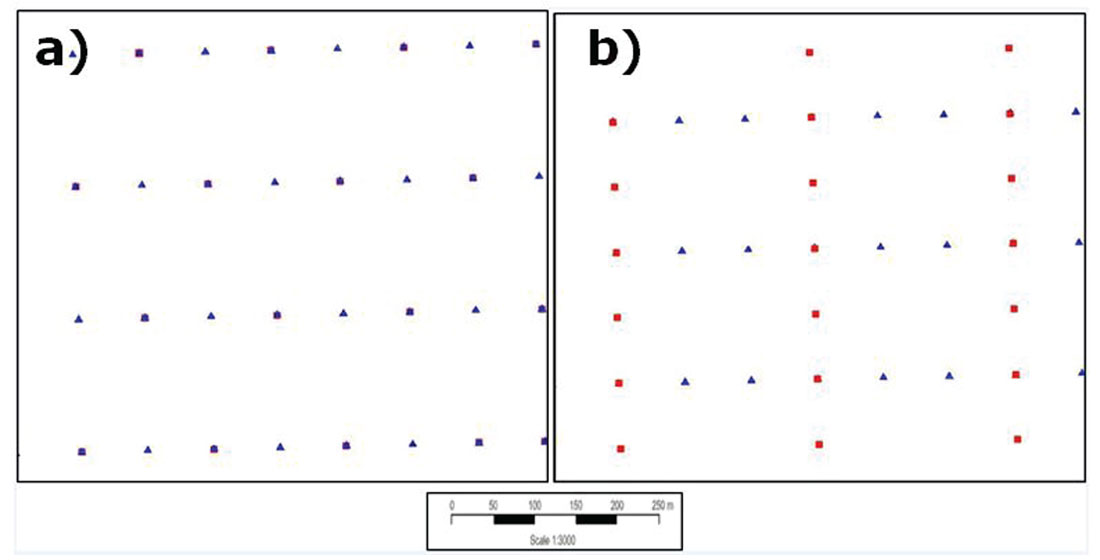
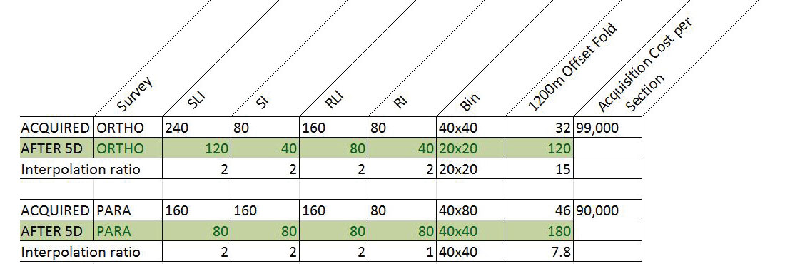
Figure 1 demonstrates the acquisition geometry in plan view for the two surveys studied and Figure 2 outlines the specific acquisition and interpolation parameters. Note a few key points from these two figures: i) the acquisition trace density of both surveys used in this study is approximately 0.01 traces/m2, with the trace density of the acquired parallel being slightly lower than the orthogonal; ii) the acquisition cost is under $100,000/section for both surveys; iii) the original natural CMP bin dimensions differ; iv) at target depth (1200m), 5D interpolation produced a 15X trace count increase for the orthogonal and a ~8X trace count increase for the parallel; and v) post-interpolation bin-sizes differed between orthogonal (20x20) and parallel (40x40) surveys in the stack displays shown later. Note that no post stack interpolation was done to avoid any additional introduction of possible errors.

Analysis between the real and the 5D data could only be done at locations where we had both real and 5D traces. Hence these comparative analyses were done only on the original grids. Also, in order to reduce footprint effects on the stacks, all stacking was binned to regular offset bins prior to mean stacking.

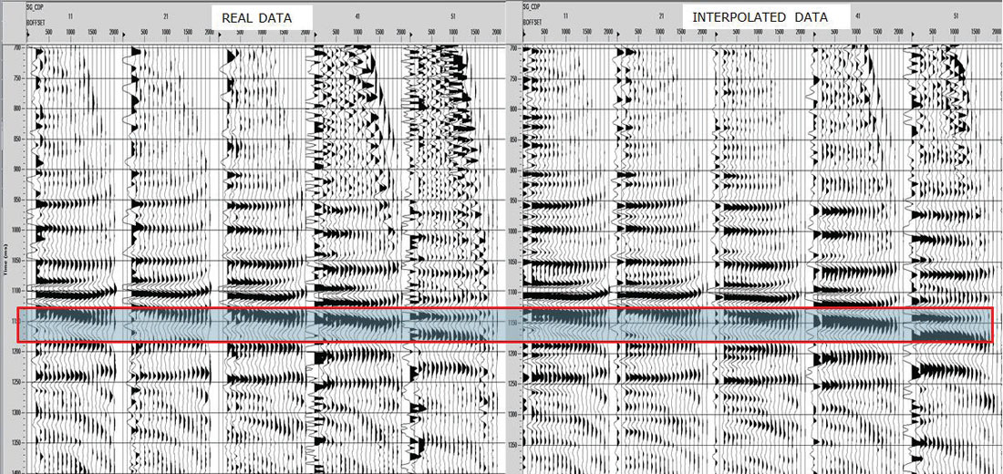
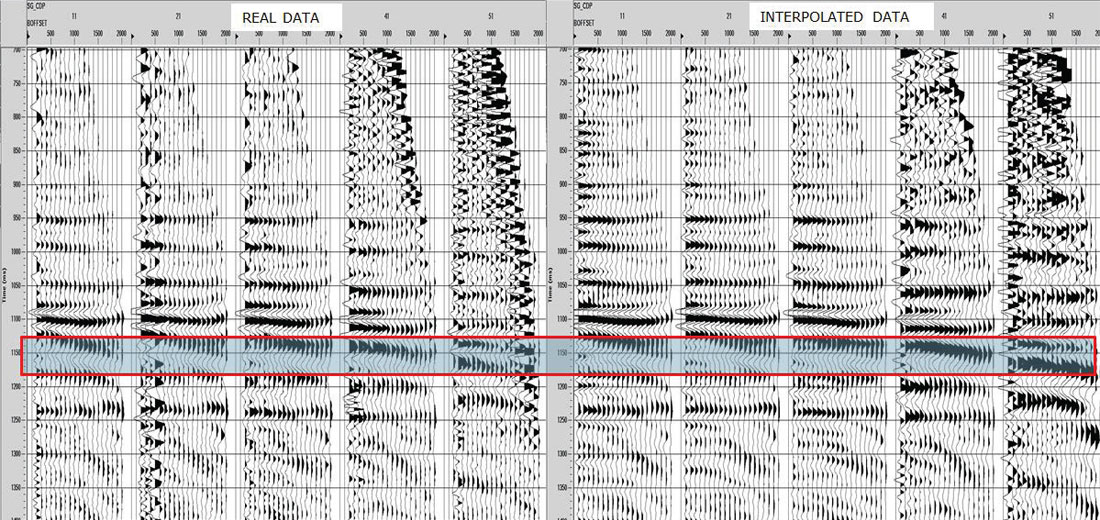
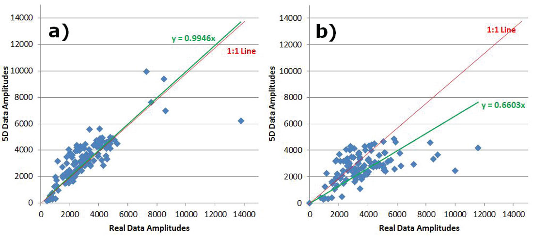
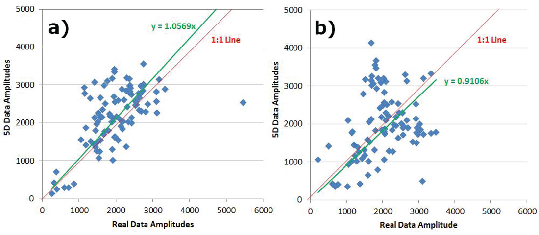
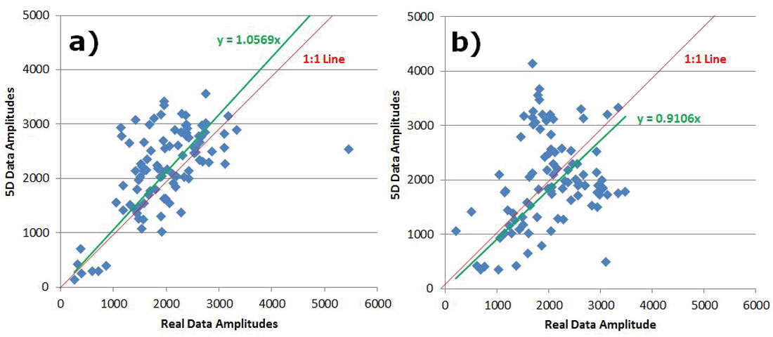
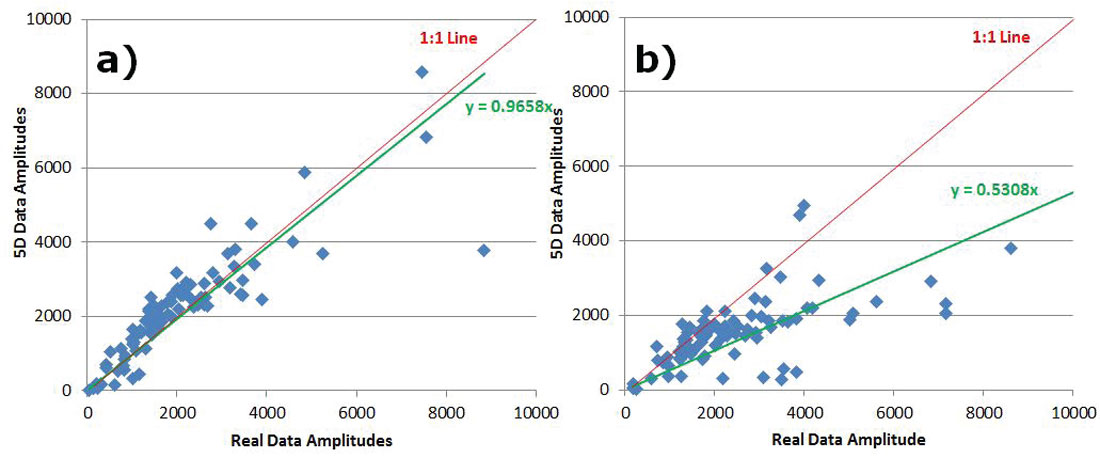
To analyze preservation of AVO attributes, five central Common Offset Stacks (COFFS) were chosen in the North-South direction on the same crossline which lies in between source lines for each survey so that no advantage was given to either one. The COFFS were generated at the same locations on both surveys by combining 5 CDPs periodically along the line binning offsets 0-2000m incrementing by 100m. The fold ratio of the 5D to real data was 7:1 on the COFF analysis for both geometries. The analysis window was around the target zone, but below the Mannville coals so that any subtleties in amplitude in the target zone were not over-shadowed by the much larger coal amplitudes (Figure 3a) and 3b)). Amplitudes were extracted on the real data and the interpolated data for both surveys. Figures 4 a) and b) show extracted amplitudes on the unfiltered data for the real and interpolated parallel and orthogonal geometries. It is clear that there is less preservation of amplitude in the interpolated orthogonal data than there is in the interpolated parallel data. For the full bandwidth, the parallel survey appears to be following Trad’s observations that ‘simultaneous interpolation in all five seismic data dimensions…has real utility in predicting missing data with correct amplitude…variations’ (Trad, 2009). Further amplitude analysis on the low end of the frequency spectrum occurs in Figures 5a) and b), and for the high end of the frequency spectrum in Figures 6a) and b). These show that the interpolation of the high frequencies is more problematic on the orthogonal data than on the parallel data; neither appears to be doing very well interpolating the low end frequencies. This was an interesting initial AVO analysis over a few selected COFFS that raised a flag that further, full-survey analysis needed to be addressed.

Extending this AVO analysis over the entire survey, a near and far offset difference method was applied. With the real and 5D gathers as input, offset-limited stacks were generated for both surveys. A window around the target zone was analyzed. The horizons that define the target zone were picked separately on each survey so as to eliminate variations in statics/phase. The near-to-far offset differences (Near- Far Diff) were calculated by subtracting the far offsets from the near offsets over the target window for the real and interpolated stacks on both the parallel and the orthogonal surveys. If the interpolator was operating perfectly, the only difference between Near-Far Diff pre-interpolation and Near-Far Diff post-interpolation should be patterned/ coherent noise associated with footprint that was successfully removed through the 5D interpolation process. Figures 7 a) and b) show the percentage difference between the real and the interpolated data’s Near-Far Diff for the parallel and orthogonal surveys respectively. 5D interpolation has correctly removed footprint, especially in the parallel case, however, it is meant to produce a dataset with regular sampling for pre-stack AVO inversion: in this particular instance, it is demonstrated that some AVO attributes are distorted through the 5D MWNI algorithm. Although both surveys have errors in interpolating AVO attributes, it is clear that over the entire survey, the orthogonal has produced interpolated data with lower percentage differences between the real data Near-Far Diff and the interpolated data Near-Far Diff that are not attributed to footprint.

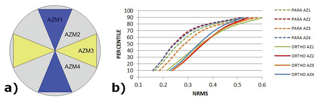
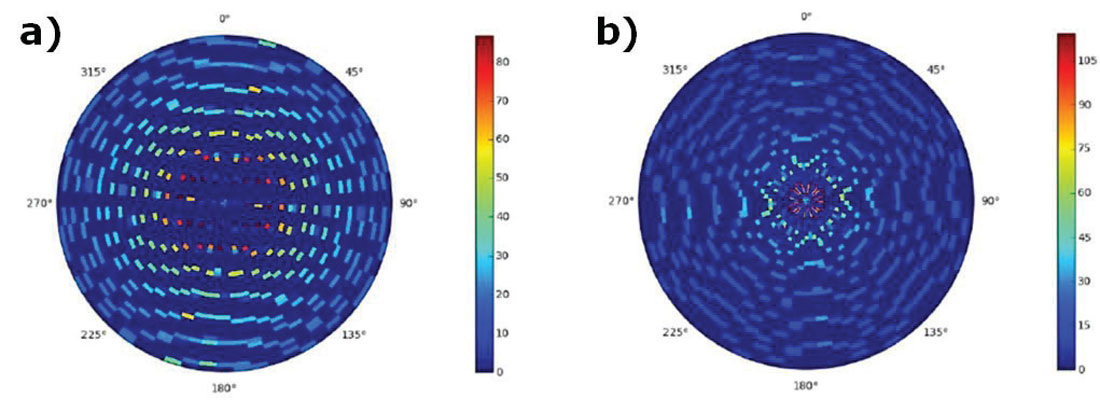
To analyze preservation of AVAZ attributes, the NRMS (a common 4D method of analysis) on the azimuthal structure stacks was used to determine if these attributes are preserved through the 5D interpolation process. The same window around the target zone was analyzed as for the AVO portion of the study and the azimuthal zones used for this analysis are shown in Figure 8 a). The fold ratio of the azimuthal stacks for the 5D to real data was 6:1 on the orthogonal and 4:1 on the parallel. We expect, in a perfectly operating 5D interpolator, that the NRMS between the real and the interpolated data be low (i.e. less than 0.6), meaning there are few differences. Figure 8 b) demonstrates that the orthogonal has only 50% of data below NRMS=0.35 whereas the parallel survey has 75% of data below NRMS=0.35. This means that the parallel survey has interpolated azimuthal gathers that are more similar to their input gathers. Figure 9 shows the rose fold diagrams for each survey’s input geometry.

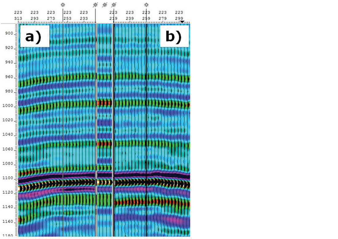
Interpreting the stacked data, the synthetic ties at the well locations were evaluated for both geometries. Near offset stacks (0-700m) were used in this analysis and no spectral balancing was applied. Figure 10 demonstrates a well tie to both the parallel and the orthogonal near offset stacks of the 5D PSTM data. There is a slight uplift in the signal-to-noise ratio in the parallel geometry, but other than that, both datasets have similar ties to geology and tie quite well to each other.

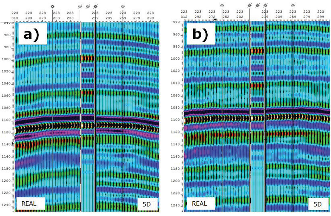
Another analysis was done on the near offset stacks comparing the real data versus the 5D PSTM data for each survey at the same well tie. It is recognized that the 5D PSTM data in this example does contain real and interpolated traces. In addition, the real data did not have PSTM applied, however, analyzing near offset stacks is a valid comparison given the lack of structure and multiples in the area. Figures 11 a) and b) show that the orthogonal survey has noisier original data to start with, however its tie to its 5D interpolated data, and to the well, are overall better than the parallel geometry’s tie.

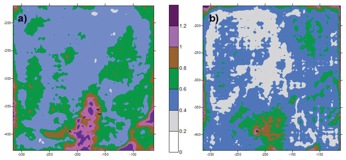
The survey-wide differences were evaluated between each geometry’s real traces versus their real plus interpolated PSTM traces to determine which geometry is best able to interpolate its acquired data. Near offset stacks (0-700m) were used in this analysis and no spectral balancing was applied. The NRMS was calculated over the zone of interest (Figures 12 a) and b)). It is obvious that the parallel survey has greater differences between the real data and the 5D interpolated data, especially in the area where source placement was challenging due to drilling constraints. The orthogonal was better able to interpolate through this noisy data area, and through the entire survey.

Conclusion

5D interpolation is a method used to regularize gathers for pre-stack processes such as inversion, AVAZ and PSTM. PSTM is an important step to condition gathers for inversion and AVAZ analysis. It is clear that knowing how 5D interpolation may have changed our data from its original form is crucial to understanding the reliability of the output from PSTM, and hence any subsequent detailed pre-stack work flows.

In this analysis, it was demonstrated that there are several methods and techniques that one can employ to compare pre- and post-interpolated data. A key point in this particular analysis is to recognize that the purpose was to examine how each geometry behaved through 5D interpolation given that each survey had its own pre-stack processing workflow for the most part. It was not tested which survey geometry best samples the actual geology. The analysis was done to demonstrate how parallel and orthogonal input data vary from their output 5D interpolated data.

It is also important to note that the surveys could be re-processed with different parameterization of the noise attenuation and 5D algorithm, and it would likely produce different results. However, much care and attention was given to the parameterization at the time of processing to optimize the results. The ability to produce high quality interpolation relies not only on the success of the processing flow prior to interpolation including noise attenuation (Sacchi and Trad, 2010), but also on the implementation of the 5D code and parameterization. 5D Interpolation is not intended to replace acquiring adequate data for processing and it must be applied very carefully so as not to introduce spurious information in a coherent manner, which stacking is unable to fix (Trad, 2009). It has been demonstrated here that there are several quality control methods that one can employ to ensure that the interpolator is behaving in a manner in which one can trust the output data.

Acknowledgements

The authors would like to thank Cenovus for permission to present the data. A special thank you to Daniel Trad and Mike Perz for their considerable feedback and comments. Thank you also to Mike for the invitation to submit a paper in this edition of the RECORDER. The authors would like to acknowledge Mauricio Sacchi for his insights around the topic of testing the output from 5D interpolation. Thank you to CGG (initial processing) and Optiseis (acquisition design) for their efforts on the data.