Real-time Induced Seismicity Forecasting and Risk Management Utilizing Research-grade Seismic Catalogs

Practical management of induced seismicity risk and effective mitigation approaches are crucial to oil and gas operations. Effective risk management procedures benefit from an accurate forecast of the largest potential magnitude event in near real-time, allowing the adjustment of operational parameters to reduce the probability of a felt or damaging event. Many models have been proposed to estimate the magnitude of the strongest possible event. Some of these models rely solely on statistics of recorded seismicity while others account for the relation of event size with operational parameters. There are also models that relate the maximum magnitude with existing geological and tectonic conditions.

In this study, we discuss different published seismicity forecasting models and evaluate their performance on a number of datasets. To understand the reliability of the various models and their sensitivity to data quality, we compare observed and forecasted seismicity for local and regional arrays. The results show that a high-quality catalog is essential to accurately forecast seismicity and drive a reliable risk management application.

Next, we evaluate the forecasting models by playing back 30+ datasets that were generated during hydraulic fracturing operations to simulate real-time monitoring conditions. We use three prediction models to estimate the maximum magnitude and one to evaluate the number of events stronger than a threshold magnitude. Our findings show that, in general, maximum magnitude estimates from different models are nearly identical and in good agreement with the observed seismicity. We also discuss the limitation of the models by examining a few cases where the seismicity forecasts were not successful. Finally, we show that over time, the forecasts lose their sensitivity to the injection volume.

Introduction

Stress changes due to subsurface fluid injection in oil and gas operations may induce seismic activity. The size and distribution of such events are a function of local geology, in situ stress conditions, and treatment parameters. Not all fluid injection operations exhibit seismicity (Shultz et al., 2018), but when they do, it is vital to monitor the ongoing induced seismic activity evaluation of the invoked risk mitigation plans.

The majority of the regulatory traffic light protocols introduced to date are based on staged magnitude thresholds, which increases the need for a better estimation of the largest magnitude event that is related to oil and gas production. Forecasting maximum magnitude in real-time is a subject of significant interest to many operators. Prior knowledge of the largest possible event in real-time allows operators to optimize and adjust their stimulation plans accordingly to prevent events that would trigger regulation-driven operational shutdowns.

A large body of work has been published on forecasting maximum magnitude (Mmax) related to fluid injection in a given area. The performance of these models has been assessed in several studies (Eaton and Igonin 2018. Shultz et al., 2018, Kiraly-Poag et al. 2016) using available datasets to identify the benefits and challenges of each method.

Shapiro et al. (2010) introduce a parameter called ‘seismogenic index’ which represents the tectonic feature of a given location and is independent of injection parameters. Using this index, cumulative injected volume, and an estimated b-value, one can calculate the number of events within a specific magnitude range and consequently determine the probability of events occurring that have a magnitude larger than the threshold magnitude that results during fluid injection (referred to hereinafter as SH10). The result from this method is valid during active fluid injection.

Shapiro et al. (2011) state that the minimum principal stress axis of the fluid-stimulated rock volume is one of the main factors limiting the probability of large magnitude events. This model essentially relates the fluid-injected Mmax with geometrical characteristics of the stimulated volume (i.e., the microseismic cloud). This method suggests real-time monitoring of the spatial growth of seismicity during rock stimulation to estimate expected Mmax and consequently to mitigate the seismicity risk.

McGarr (2014) develops a simple relationship between the cumulative volume of injected fluid and the largest seismic moment. This model is developed based on some assumptions, including a fully saturated, brittle rock mass with a b-value of 1.0.

Van Der Elst et al. (2016) demonstrate that the size of the strongest events from seismic activities related to fluid injection is consistent with the sampling statistics of the Gutenberg-Richter distribution for tectonic events. They conclude that injection controls the nucleation but that earthquake magnitude is controlled by tectonic processes. They introduce a model based on this hypothesis (referred to hereinafter as VDE16_Seis). They further link their model to total injected volume and seismogenic index (referred to hereinafter as VDE16_SI-V).

Eaton and Igonin (2018) add a tapered Gutenberg-Richter relationship to VDE16_Seis, to introduce a limit to the size of the maximum magnitude event.

In this paper, we calculate the seismicity for regular time intervals (e.g., Kiraly-Proag et al. (2016)) utilizing the SH10, VDE16_Seis and VDE16_SI-V models to illustrate how well the techniques forecast Mmax and the number of events in near real-time based on recorded seismicity and treatment data. Other than the three models used in this study, we investigated three other published methods and decided not to utilize them in the forecasts. Shapiro et al. (2011) do not account for the far-field triggering due to poroelastic stress effect and neglect nucleation of an event in the stimulated volume while the fault continues out of the events cloud. Our analyses show that McGarr (2014) overestimates Mmax compared to the observations. Furthermore, this model is developed based on assumptions including a constant b-value of 1. Eaton and Igonin (2018) limit upper magnitude level in the real-time application, which we did not prefer.

In order to improve the practicality of seismicity forecasts, all observations and estimations are presented in an interactive dashboard environment with the objective of providing effective real-time operational risk mitigation feedback.

Case Studies

While not shown in this paper, we test the dashboard on 30+ datasets from hydraulic fracture (HF) operations. In general, there was a very good agreement between observations and estimations across the various datasets. The following three case studies highlight a key common point that was observed in each playback. The case studies are related to three HF monitoring operations in Western Canada.

Case Study I illustrates how the models result in seismicity estimations that are very close to the observations. The results from this case study are typical and represent the majority of the playback datasets where a rich and accurate catalog was collected using either a local array or a near-regional network with advanced processing. Case Study II demonstrates the impact of treatment data in the forecasts. Lastly, Case Study III demonstrates a limitation of the algorithms. We summarize results for each dataset in a dashboard environment.

Case Study I uses data acquired during a 36-day monitoring period from an 11-station local surface-monitoring array located in Alberta. All stations were located within 8 km of the pad. The array recorded 2374 events during the monitoring period, with local magnitudes ranging from ML-1.1 to ML2.6. The b-value computed for the entire catalog was 0.9, which is consistent with the Gutenberg-Richter relationship for natural seismicity with the magnitude of completeness (Mc) of ML-0.6.

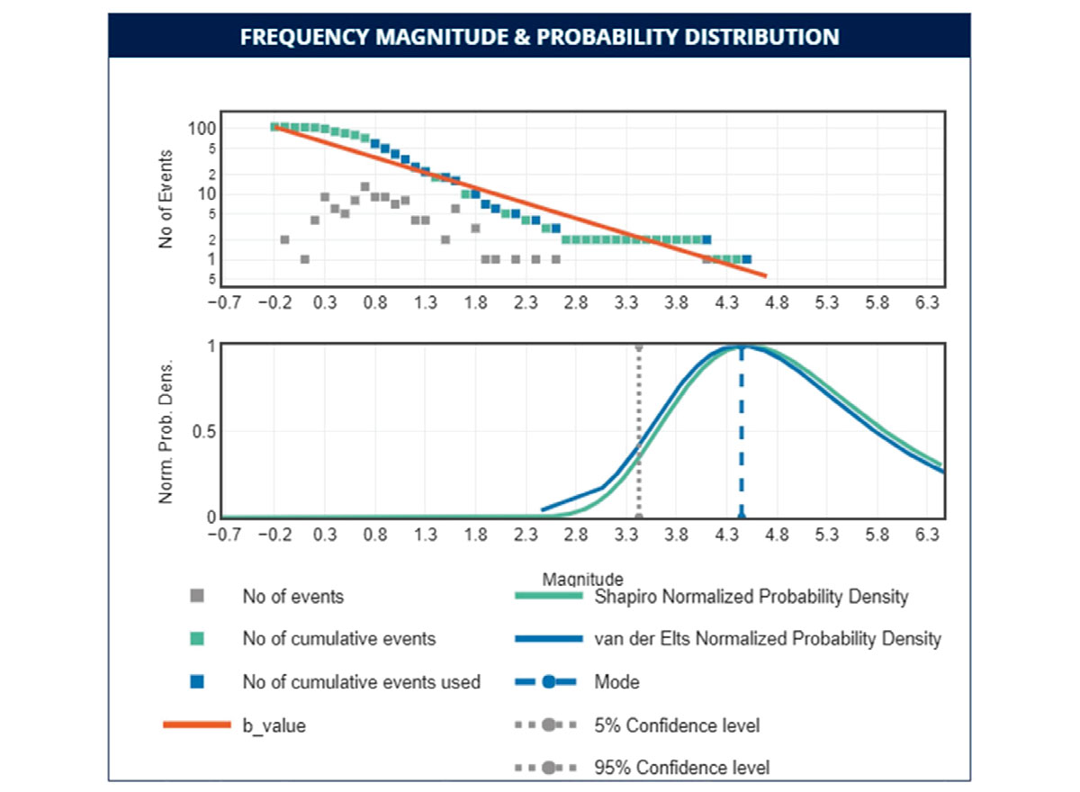
Figure 1 is the dashboard for Case Study I. Figure 1a shows the Gutenberg-Richter distribution on top and the normalized probability density function from SH10 (green line) and VDE16_Seis (blue line) on the bottom. The vertical dashed line is the mode of the VDE16_Seis probability density function and the dotted lines denote 90% confidence bounds of the distribution. Figure 1b illustrates the forecasted Mmax gauge on top and the probability of exceeding magnitude ML2.5 gauge on the bottom. The 3D events distribution is displayed in Figure 1c.

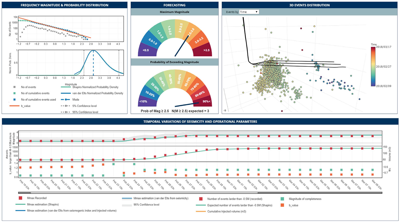
To simulate real-time monitoring, we play back the data and calculate the b-value and Mc at regular time intervals from the cumulative seismicity data. We use these parameters to estimate the expected Mmax and the number of events that exceed a threshold magnitude at each time step and compare them to the recorded seismicity. It should be noted that the estimated Mmax is the mode of the probability density function (Figure 1a). The symbols in Figures 1d show results at 12-hour intervals over the stimulation period. On the top plot, the recorded (red squares) and estimated Mmax (green and blue lines) are shown over time. The middle plot presents the recorded number of events that are larger than the threshold magnitude of ML-0.5. The bottom plot in Figure 1d shows the time-varying estimation of b-value and Mc. As more events are detected, the Mc and b-value become more stable. In this example, we observe a very good agreement between the recorded and estimated seismicity including Mmax and the number of events.

Next, we examine the impact of the seismic catalog quality on the risk management application. This dataset was recorded by a 20-station regional backbone array around the well pad from Case Study I. The location of the stations ranged from 3 km to 72 km from the pad. The regional array detected and located 80 events in the same time period that had poor location accuracy in comparison with the locations from the local network (Case Study I). The completeness and accuracy of this catalog is not sufficient for statistical analysis and would result in large probabilistic prediction uncertainties.

This example emphasizes that a research-grade catalog is an essential requirement for driving a reliable risk management application. A local or near-regional seismic monitoring resolution along with advanced seismic data processing techniques is required to generate data sets that are both rich enough and accurate enough to be used as inputs in real-time seismicity forecasting models. However, to accurately compute cataloglevel data products (such as b-value or seismicity rate variations), the seismicity catalog must be extended with small magnitude events that are well below the regulation threshold. Additionally, the event locations should be highly accurate in order to enable the delineation of activated structures.

We next investigate the impact of cumulative injection volume data on the forecasted seismicity parameters. We discover that estimations of maximum magnitude and the number of events lose their sensitivity to the variation of cumulative injection volume over time. Following Kiraly- Proag et al. (2016), we reevaluate b-value, Mc and seismogenic index in every time step, taking into account the cumulative injection volume and the cumulative recorded seismicity from the current time. Then these parameters and the designed cumulative injection volume data from the next time step are used to forecast the seismicity. The relationship between Mmax and cumulative volume can be seen in the form of equation 1:

As cumulative injection volume grows in time, the logarithm of the ratio of current cumulative injection volume to the cumulative injection volume at the next time step reduces, and as a result, the Mmax estimation is not very sensitive to changes in the total injection volume.

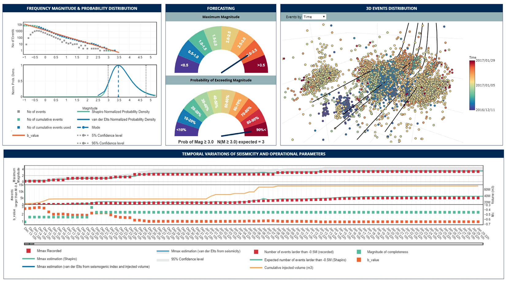
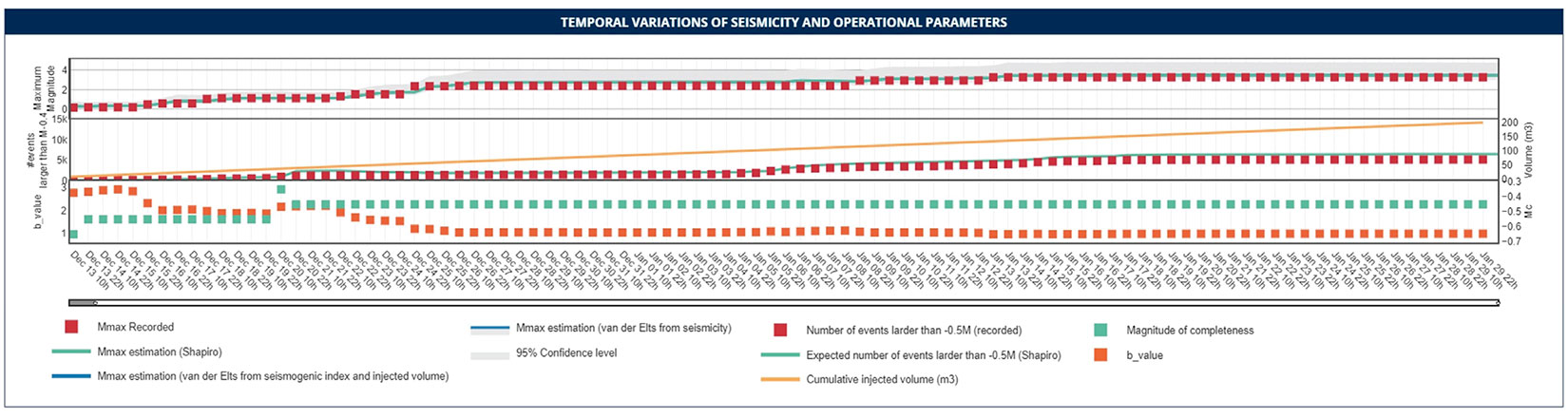
Case Study II illustrates the impact of cumulative injected volume on the forecasts. It consists of data that was recorded on a 9-surface-station local network acquired over a 45-day period. In addition, there are 68 shallow borehole sensors that recorded for four days. In total, 7778 events are in the catalog with magnitudes ranging from ML-0.9 to ML3.2. To test the impact of cumulative volume data on the estimated seismicity, we reevaluate all parameters with and without considering the real cumulative injection volume. Figure 3 shows the dashboard for Case Study II. Figure 3d presents the observations and forecasts over time when we include the real cumulative injection volume (orange line in the middle panel). Figure 4 shows the forecast values using a constant injection rate. A comparison of the estimated maximum magnitudes and the number of events from Figure 3d and Figure 4 demonstrates the limited impact that injection volume data has on the forecasts. Additionally, it demonstrates the lack of correlation between the cumulative injected volume and the observed seismicity.

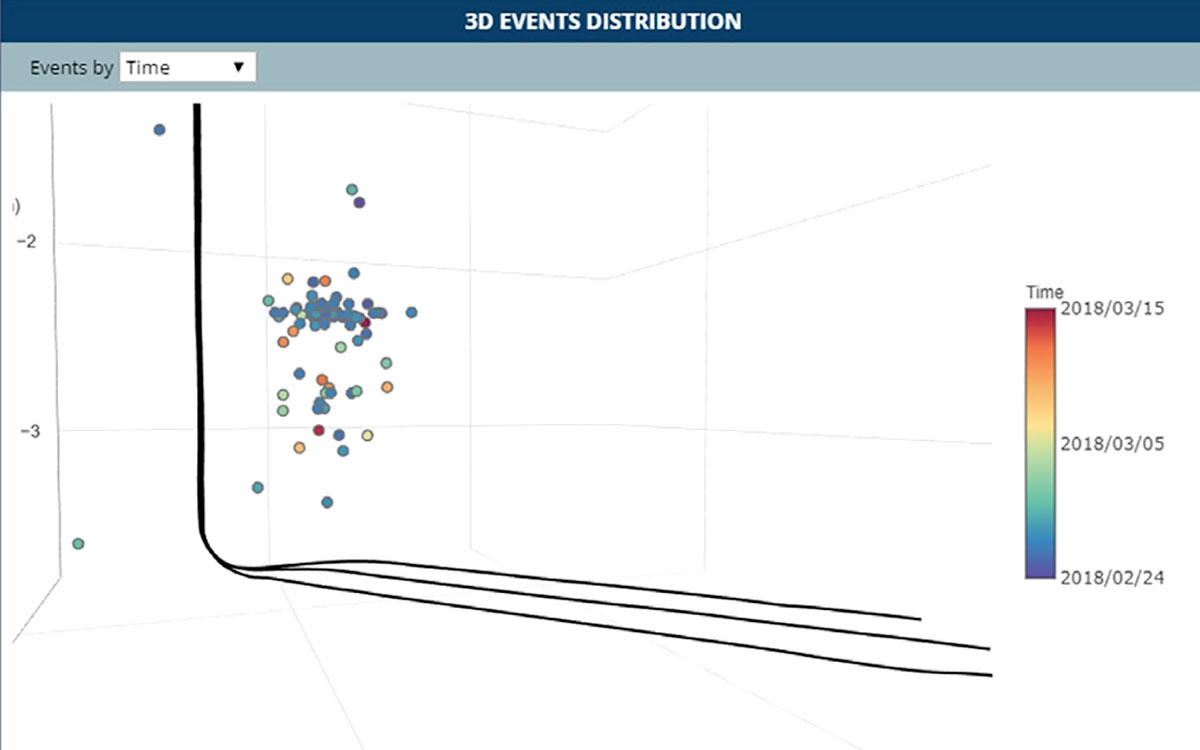
Case Study III demonstrates one of the main limitations of the forecasting models. The dataset is from a 4-station local induced seismicity monitoring array of a hydraulic fracturing operation over a 2-year period near Crooked Lake, Alberta. Figure 5 illustrates the seismicity and statistical analysis of this data set over 50 days when the seismic activity was highest. The analysis was performed on 12-hour intervals. The final results show a good agreement between the expected and recorded Mmax with a b-value of 0.69 from a well-behaved Gutenberg-Richter distribution. However, a closer look at the time when the strongest event happened shows that the models were not successful in forecasting the large event which occurred early in operation.

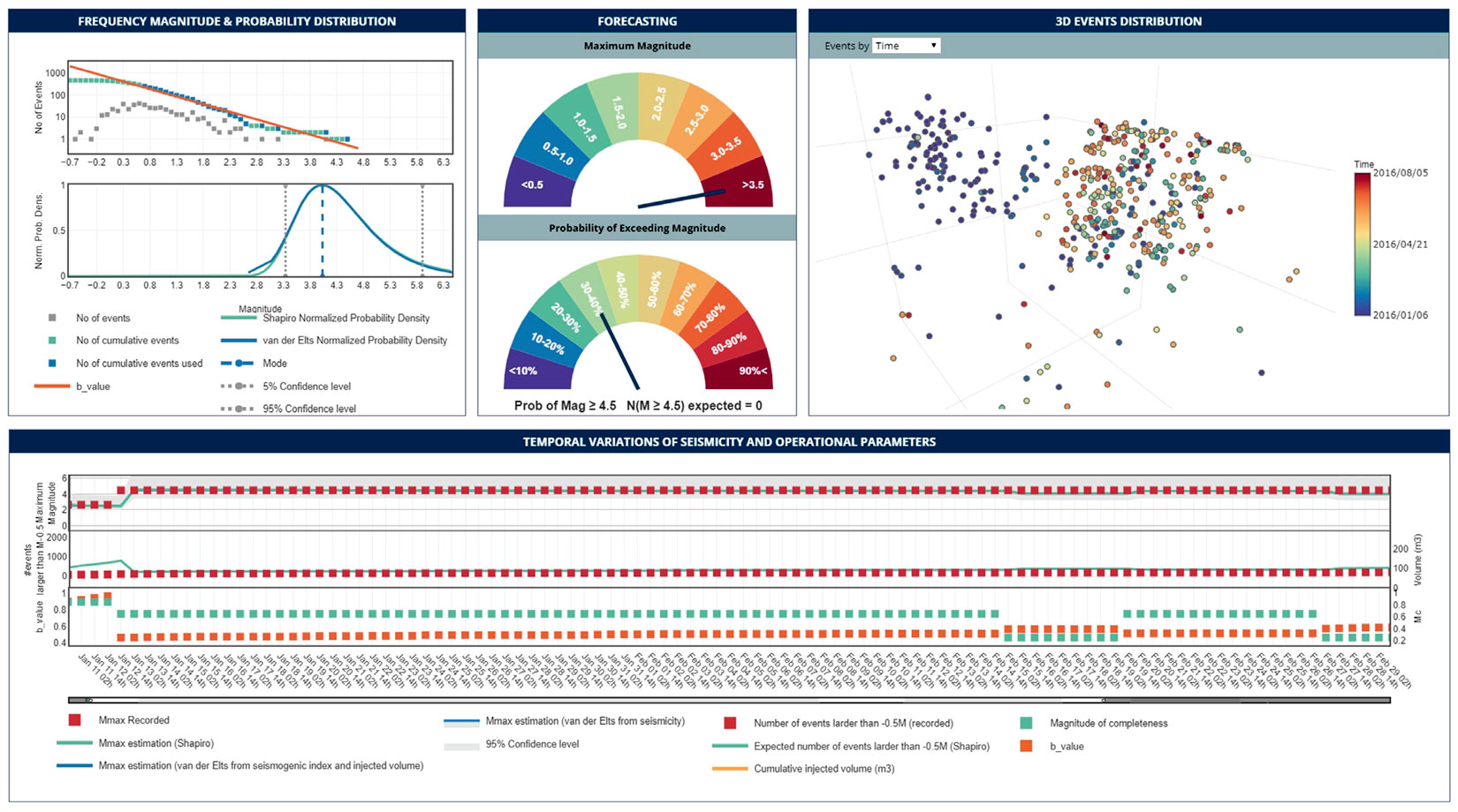
Figure 6a is a snapshot of the seismicity related to the first few days after starting injection when 85 events were recorded. The estimated b-value from the available data is 0.97. Using the recorded seismicity catalog, the models predicted that the maximum magnitude interval with 90% confidence should fall between ML2.0 to ML3.9. The mode of the maximum magnitude probability density function is ML2.5; six hours later an event with ML4.5 occurred. Figure 6b shows the seismicity after the ML4.5 event. The forecasting result prior to this event shows a very small likelihood (1.15%) for the occurrence of such a large event.

This example highlights the limitation of forecasting models using statistical approaches when a large event occurs early in the operation. The sample size hypothesis holds that each event in the sequence has the same probability of occurrence and that the order of occurrence of the largest earthquake is random within the sequence (Van Der Elst et al. (2016)). In other words, induced earthquake magnitudes are drawn independently from a Gutenberg-Richter distribution rather than being physically determined by increasing injection volumes. As a result, the large event can occur anywhere within the sequence, including at the beginning.

Discussions and Conclusion

Induced seismicity risk can be evaluated prior to drilling by detailed geological and geophysical analysis of seismic data to characterize the pre-existing structures and potential fluid pathways to those structures. Drilling and completion programs can then be designed to minimize the likelihood of proximal faults activation and large magnitude event occurrence. However, as the data recorded to date in Western Canada has shown, most of the activated faults are unmapped and the conditions (in situ stress state, fault proximity, area, and fault orientation) at each pad are highly variable. This is witnessed by the observation of different activation mechanisms and the presence of, in some cases, seismicity that is not associated with known faults. These observations highlight the importance of real-time seismic monitoring in understanding, evaluating, and managing the seismic risk in near real-time.

In this study, we evaluate the performance of the approach proposed by Shapiro et al. (2010) and two models from Van Der Elst et al. (2016) for estimation of Mmax and number of events. The results from our analysis were presented in dashboard format as part of a real-time feedback loop to the operational risk mitigation protocols.

The summary of our observations is as follows:

• Our analysis confirms that the estimated seismicity from different models agrees well with the observed seismicity in terms of largest magnitude and recorded events in most cases.
• We observe that the estimated maximum magnitude from three models are very close in all test cases.
• The cumulative injection volume has low to no impact on forecasted seismicity, and over time, the forecasts lose their sensitivity to the cumulative injection volume.
• We observe some scenarios in which a strong event occurred in early stages of the HF operations, resulting in under-prediction of Mmax.
• The quality of the seismicity catalog has a significant effect on the outcome of the forecasting model. A high-resolution data set recorded by either a local array or a near-regional network with advanced processing is a requirement for this analysis.
• It is worth noting that the three forecasting models used in this study were developed based on moment magnitude. Consequently, prior to applying the models, the seismicity catalog should be homogenized by converting all magnitude types to moment magnitude.

The seismicity forecasting models are presented as a dashboard in this study which can provide operators a measure of whether the current injection parameters may cause a strong event in near real-time. This is the first version of the dashboard. Hence, adjustments to the displayed parameters and the forecasting models are expected in the near future. The value and accuracy of predictions will improve with time and continuous feedback from operational use.

Acknowledgements

We are grateful to our colleagues at Nanometrics Inc. for their support and contribution to this study. In particular, we would like to thank Andrew Reynen, Ben Witten, Emrah Yenier and Christine Cowtan. We would like to acknowledge Repsol and two anonymous operators for granting permission to publish on data obtained from their local networks.