Quantitative Comparison of Inversion Methods for Estimating Density from Seismic Data

In the Athabasca oil sands, lithology and fluid composition are typically better correlated with density than with other elastic properties, such as P- or S-wave velocity. Therefore, improving the accuracy of density estimates in oil-sands reservoirs has become one of the most important goals in quantitative interpretation, which integrates seismic, well-log and geological data through deterministic or stochastic inversion methods.

In this paper, we applied three methods for density estimation to an oil-sands reservoir in the Athabasca oil sands area; specifically, these are:

1. PP pre-stack AVO inversion;
2. PP-PS joint pre-stack inversion;
3. multi-linear regression.

Direct comparisons of estimated density, as determined using the above three methods, were made to evaluate the predictive ability of each method, and to quantitatively demonstrate the value added by PS data. Predicted density from each method was cross-corelated with measured density logs from 113 wells; the correlation coefficients are 63% for PP-inversion, 81% for PP-PS joint inversion, approximately 90% for a step-wise regression method. Additionally, the top three of four attributes contributing to density estimates from multi-linear regression were found to be from PP-PS joint inversion. Therefore, we can conclude that the PS data has improved density estimates and thus played an important role in refining density predictions.

Introduction

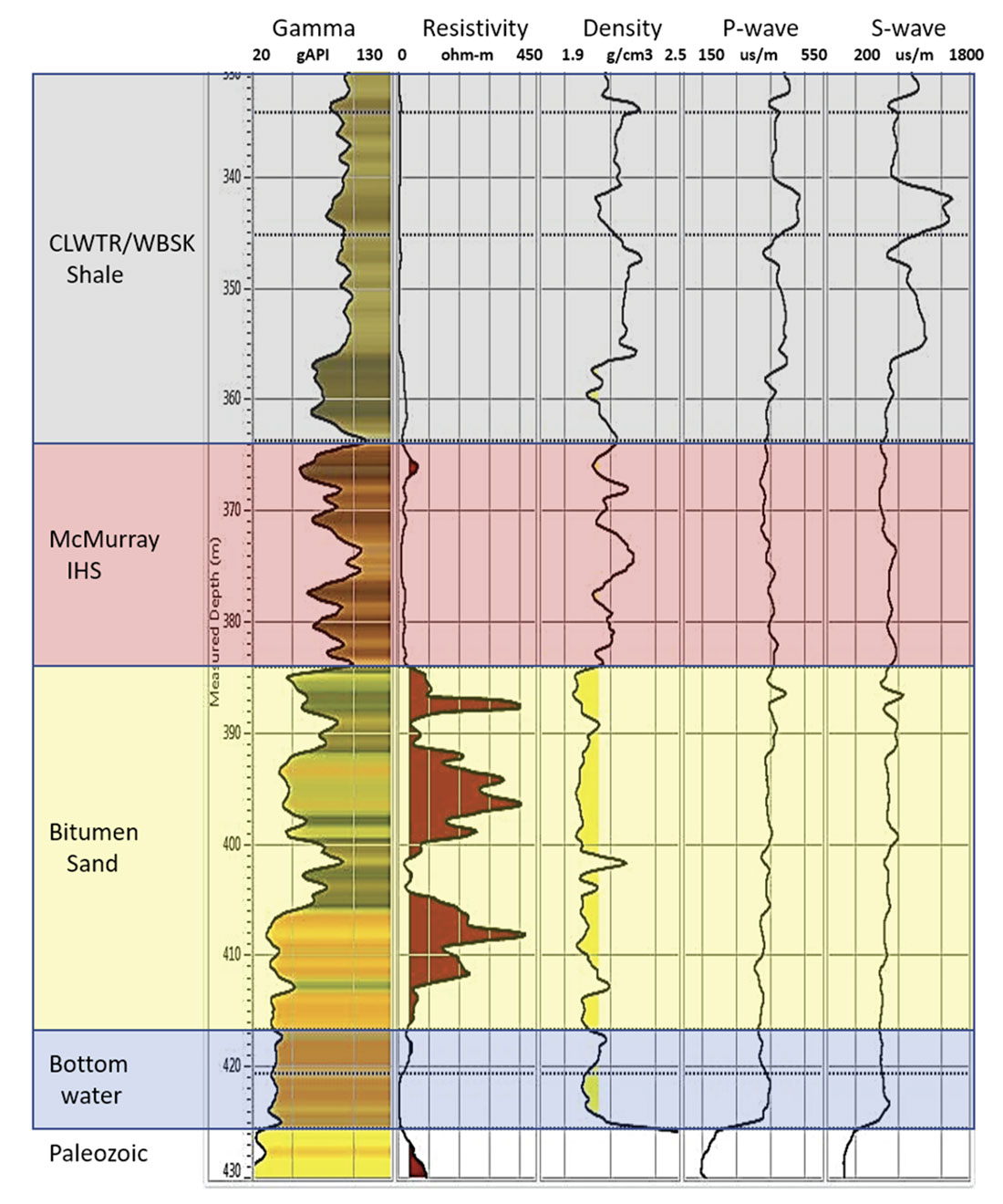
The main reservoir in the Athabasca oil sands area is the Cretaceous McMurray Formation. In this study, the McMurray Formation has been subdivided into three lithofacies:

1. clean sand;
2. inclined heterolithic strata (IHS);
3. mudstone / shale.

Figure 1 shows a characteristic log suite through the McMurray Formation within the study area. Lithofacies within the McMurray Formation are commonly variable, both vertically and laterally (see Hein et al., 2000). The scale of heterogeneities in the McMurray formation ranges from millimeters in IHS lithofacies, to many meters on a reservoir scale. Intra-reservoir heterogeneities, meaning mudstone/shale units thicker than a few meters, are significant considerations in well placement design because they act as baffles to steam chamber development. Seismic imaging is an important tool in identifying these zones.

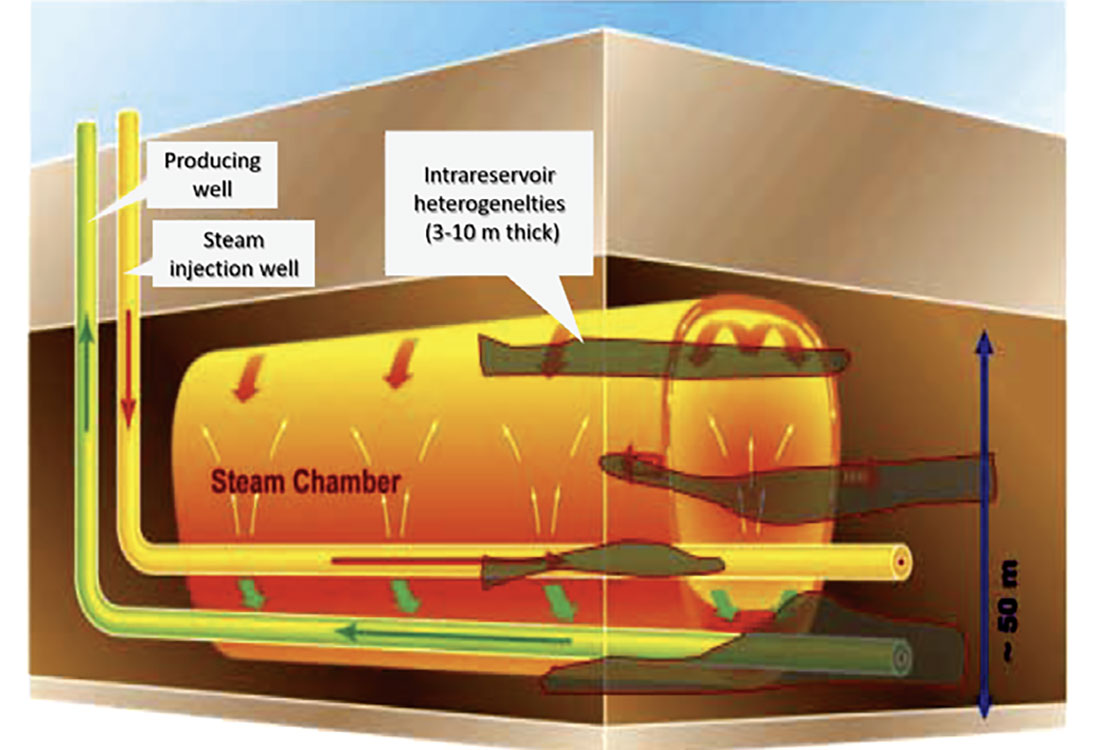
Steam assisted gravity draining (SAGD) is a production method that uses paired horizontal wells to extract bitumen (Figure 2). The producing well is first drilled within the reservoir, then a second well (the injector) is drilled a few meters above. Upon completion, steam is injected into the injector well, which mobilizes bitumen, causing it to gravitationally drain into the producing well, from which it can be pumped to the surface.

Why density?

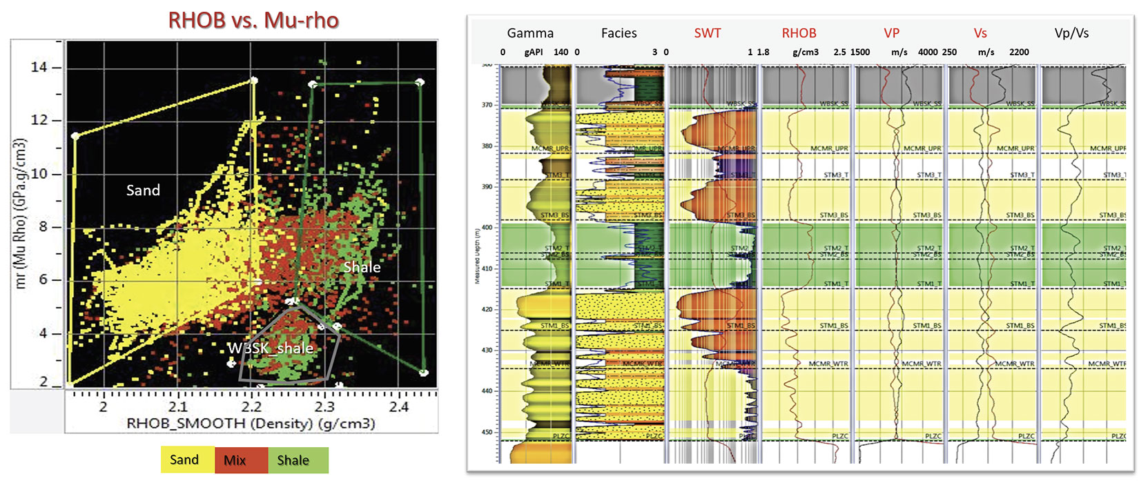
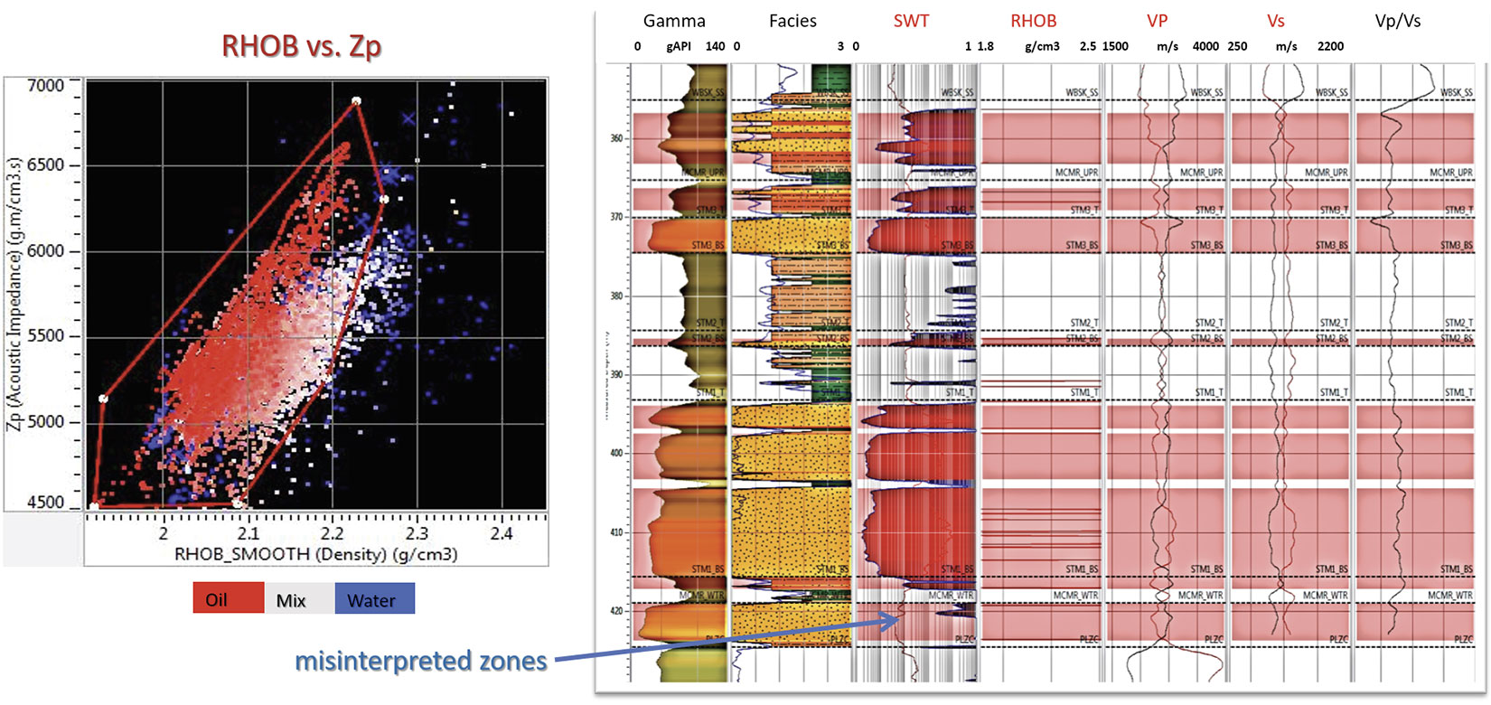
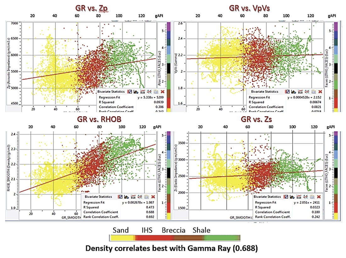
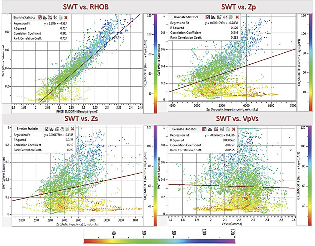
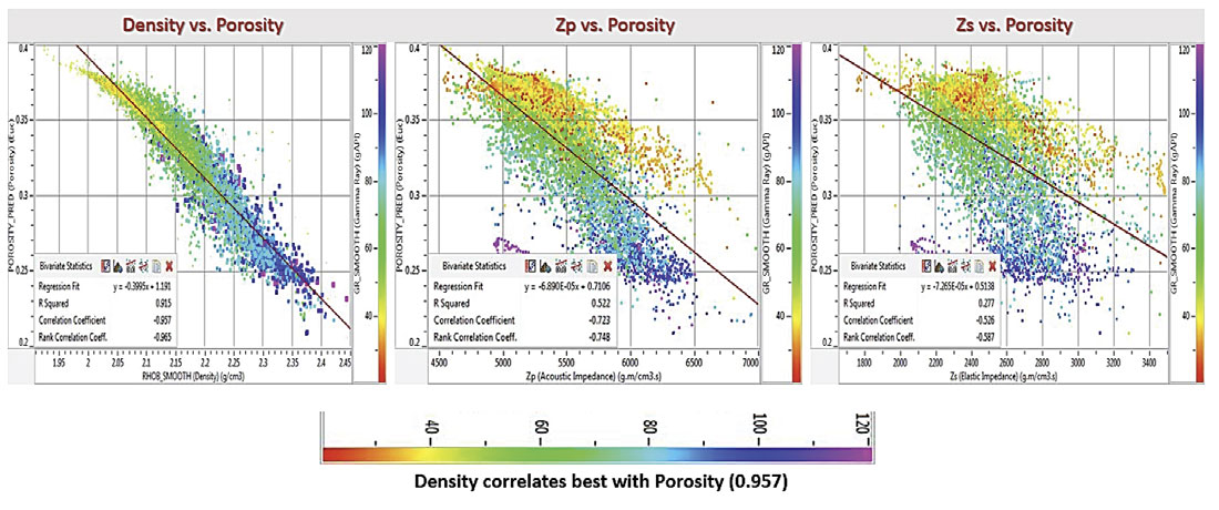
Rock physics analysis of the dipole sonic logs in the study area suggests that bitumen-saturated sands have lower densities than surrounding IHS or shale zones, and can be differentiated on a density vs. mu-rho cross-plot (Figure 3). Bitumen can also be distinguished from water (not including bottom water) on a density vs. P-impedance cross-plot (Figure 4). Overall, the best correlation coefficients with gamma (lithology), water saturation (fluid composition) and porosity are found with density, as compared to other elastic properties (P- or S-wave velocity; see Figure 5).

Therefore, in Athabasca oil-sands reservoirs, improving the density estimates is one of the most important goals of seismic inversion.

We applied three approaches to a study area within the Athabasca oil-sands region. Specifically, these approaches are: 1) PP pre-stack AVO inversion, 2) PP-PS joint pre-stack inversion and 3) multi-linear regression.

Methods

1. PP pre-stack AVO inversion method

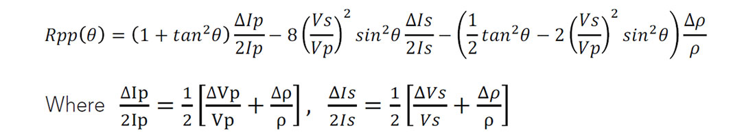
Density extraction from P-wave inversion is based on three-term AVO theory. The three-term P-wave AVO approximations from Fatti et al. (1994) is given as:

This approximation is used to estimate P- and S-impedance and density from a linearized approximation (Simmons and Backus, 1996; Hampson et al., 2005). It suggests that a wide aperture of reflection angles (> 40°) is required to achieve a stable density estimates.

The Athabasca oil-sands reservoir is relatively shallow, located at between 200 and 500 meters depth. Modern acquisition methods are often designed to cover a wide-angle range. Additionally, with the advent of new processing technologies, which include regulated binning and VTI/HTI anisotropic correction in pre-stack migration methods, density estimates from P-wave AVO inversion become feasible. Gray et al. (2004) and Roy et al. (2008) have demonstrated that reliable density estimates can be obtained using wide-angle P-wave AVO inversion by correcting for anisotropy on the gathers.

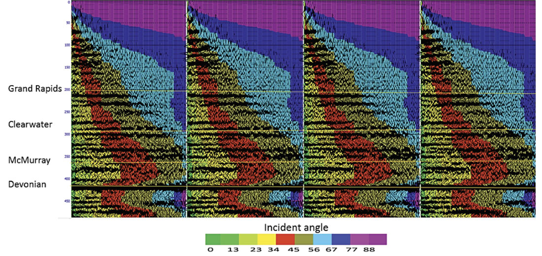
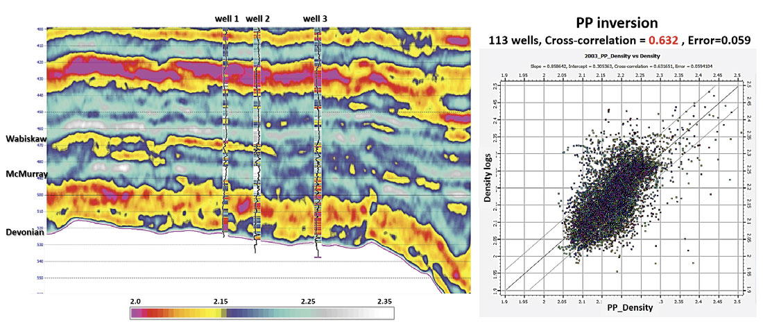
Figure 6 shows the input PP AVO gathers used for P-wave inversion. The valid angle range reaches about 40° at the zone of interest. Figure 7 shows density predicted from P-wave three term AVO inversion. The section intersects three well locations. The superimposed density logs of these three wells show a fairly good prediction at wells 1 and 2, however some thin layers appear to have been missed at well 3; reservoir thickness was also under-predicted at the third well location.

The correlation coefficient between predicted density volume and measured density logs (n=113 wells) is 0.63., which is considered to be a reasonable density estimate from PP data.

2. PP-PS joint pre-stack inversion method

The PS AVO equation of Aki and Richards (2002) shows that the converted PS gathers are related to density and shear reflectivity:

Where α is the compressional velocity, β is the shear velocity and ρ denotes density. The angle i is the average of incident and transmitted P-wave angles while j is the average of reflected and transmitted S-wave angles. Theoretically, there are fundamental advantages to estimating density from multi-component data, as compared to conventional P-wave AVO inversion methods. Firstly, wider PS angle coverage is expected for a given incident angle range because of the slower velocities of S-waves, compared to the corresponding P-waves (Gray, 2003). Secondly, having another source of shear velocity and density information derived directly from PS data should stabilize inversion and reduce the uncertainties and challenges associated with the P-wave AVO gradient and intercept method. Finally, because shear velocity is sensitive to changes in lithology, but not fluid composition, multi-component methods may show better results in where lithology and fluid composition each vary. However, the joint PP-PS inversion has not been widely applied and appreciated for several reasons. Firstly, additional costs are incurred for multi-component seismic survey acquisition, processing and inversion. Secondly, PS data is naturally lower in frequency and signal-to-noise-ratio; thus, the registration of PS events to PP events and joint inversion can be a challenge, and as a consequence the difference in estimates from PP-PS joint inversion and from PP pre-stack inversion may only be subtle.

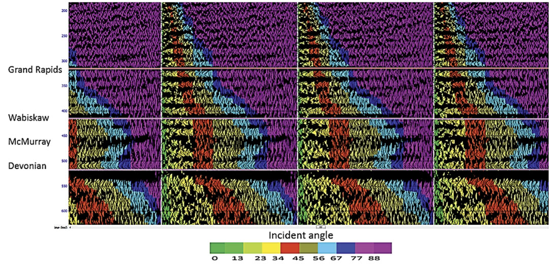
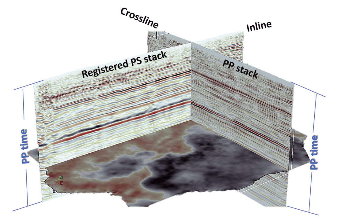
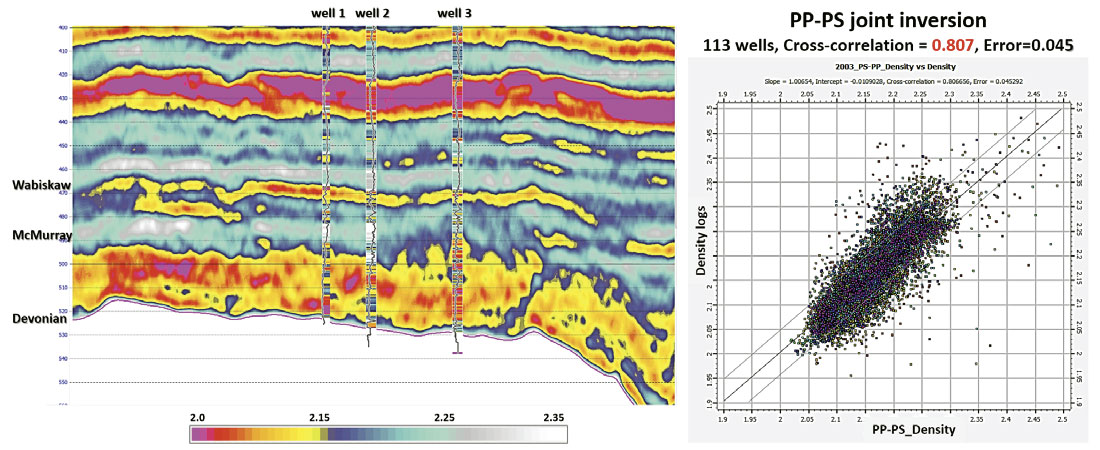
The data used in this study include acceptable PS data (up to 40 Hz in frequency and up to 65 degrees in angle in the zone of interest (Figure 8)). PS to PP registration was done in three major steps: First, dipole sonic logs were used to correlate both PP and PS data. Then, four major geological markers were picked for each volume independently and used for event matching. Finally, both PP and PS-in-PP time volumes were loaded in 3D view (Figure 9), with PP in inline direction and PS-in-PP time in crossline direction, allowing for comparison of the phase and geological markers through the whole volumes and for final manual adjustment if necessary. Density estimates from PP and PS joint inversion are shown in Figure 10. Compared to PP inversion results (Figure 7), density prediction is improved at the third well and to the west; the results also show more continuity in the bitumen reservoir and in the caprock above the McMurray Formation. The correlation coefficient is about 81% between predicted and measured density from 113 wells, meaning there is an 18% improvement compared to the results from PP AVO inversion.

3. Multi-Linear Regression (MLR)

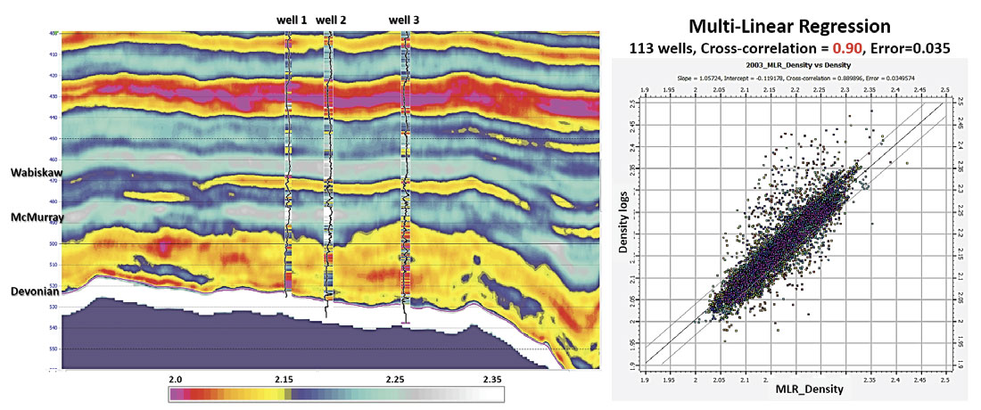
To further increase the vertical resolution and refine the prediction, a step-wise linear regression method was used to predict density through a statistical relationship derived between seismic attributes and target well logs (Hampson et al., 2001). This statistical method works very well when one has ample well control and many well-correlated seismic attributes, as is often the case in oil-sands reservoirs.

The example below covers 113 vertical wells within area of 2 km², 18 seismic attributes from PP and PS stacks, AVO products, PP inversion and PP-PS joint inversion results. Table 1 shows the results of step-wise regression; the top four attributes are:

1. PP-PS density;
2. PP-PS P-impedance;
3. Integrate of seismic;
4. PP-PS mu-rho.

Figure 11 shows the density estimate from the MLR method. A correlation coefficient of 0.90 was observed. Measured uncertainty (as shown by error bars) also decreased from 0.059 (PP inversion) to 0.045 (PP-PS joint inversion) and reached 0.035 with the MLR method.

Conclusions

Three inversion methods were used to predict density volume. The results for each method have been compared with well data from 113 wells. The correlations between predicted and measured density logs improved from 63% with PP inversion to 81% with PP-PS joint inversion, and measured error decreased from 0.059 g/cc to 0.045 g/cc. Density estimates from PP-PS joint inversion show improvement over PP inversion, especially where P-data do not have wide angle coverage (< 30°) and do not show strong reflections, which may be related to subtle contrasts in reservoir properties (encompassing both lithology and fluid variations). Adding an additional ~20° angle coverage and having another source of density estimates from PS data could stabilize inversion predictions and reduce the uncertainties associated with the P-wave AVO method.

The MLR method was applied last in order to refine the density prediction by integrating the inversion results from both methods with well data. It appears to show the best correlation (90%) and smallest error (0.035 g/cc). However, the top three of four attributes contributing to the density prediction are from PP-PS joint inversion results. Therefore, we can conclude that PS data has improved seismic density prediction.

Acknowledgements

The authors thank Devon Canada for permission to publish this work. Special thanks to Glenn Larson and George Thomson for their support.