Programming a Seismic Program

Programming is becoming an increasingly useful skill for the modern geoscientist. I don’t mean to suggest that all geoscientists should become software developers and start making full-blown desktop software applications. But programming can and will super-charge your work, making you more productive and more thorough. We can write code to outline a problem, design tests, collect or compute data, or to execute large, repetitive tasks, freeing us to ask questions. Sound programming practices share the same qualities that we hold in high regard as scientists and technologists: work that is well-documented, reproducible, testable, and verifiable for correctness and accuracy.

In this article, we’ll design a 3D seismic survey in order to frame some of the principles of scientific computing and programming. We’ll cite a small amount of code in Python throughout the text to bring attention to some key steps in the process.

The race for useful offsets

One of the factors influencing the pattern of sources and receivers in a seismic survey is the range of useful offsets over the depth interval of interest (Cooper, 2004). If the area to be imaged has more than one target reflector, you’ll have more than one range of useful offsets. We can model the shape of major reflectors starting with an estimate of a root-mean-squared (RMS) velocity profile or interval velocity profile from sonic log (Figure 1).

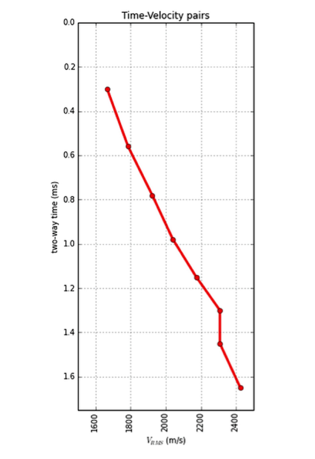
For shallow targets, this range is limited to near offsets, due to direct waves and first breaks. For deeper targets, the range is limited at far offsets by energy losses due to geometric spreading, moveout stretch, and system noise.

In seismic surveying, one must choose a spacing interval between geophones along a receiver line. If phones are spaced close together, we can collect plenty of samples in a small area. If the spacing is far apart, the sample density goes down, but we can collect data over a bigger area. So there is a trade-off and we want to maximize both; high sample density covering the largest possible area.

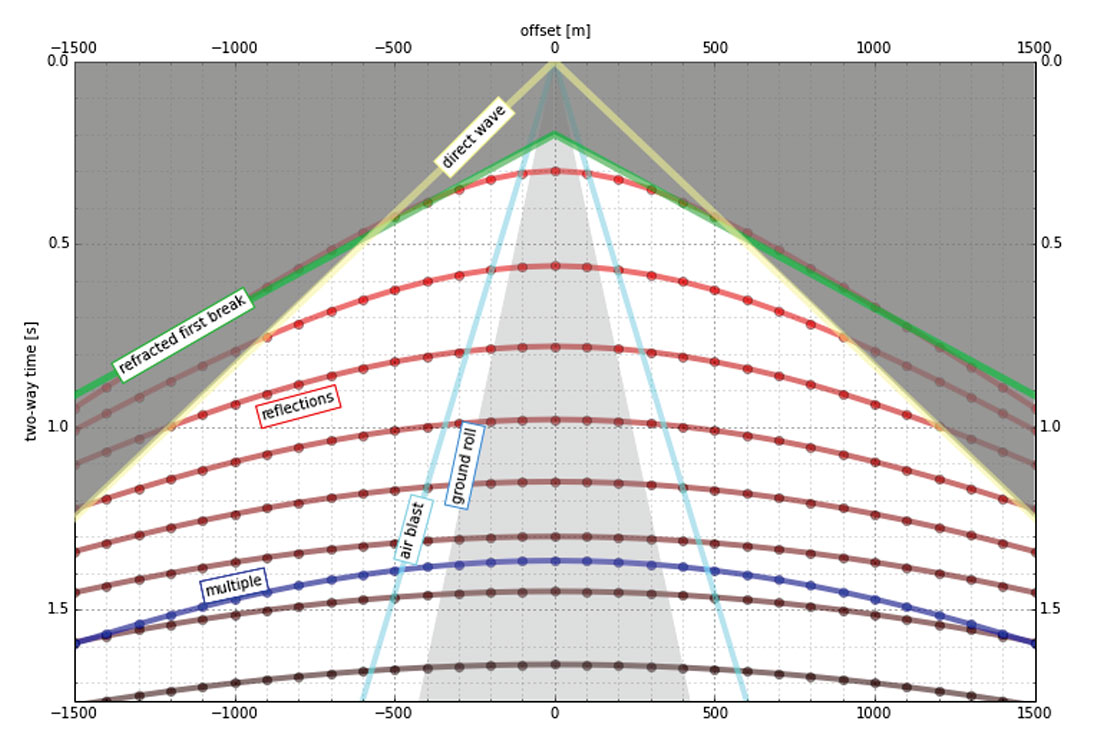
It isn’t immediately intuitive why illuminating shallow targets can be troublesome, but with land seismic surveying in particular, the first breaks and near surface refractions, which are used to determine statics, clobber shallow reflecting events (Figure 2). In the CMP domain, the direct arrivals show up as linear events, which are eventually discarded by the so-called top-mute operation before stacking or migration. Hyperbolic reflection events that arrive later than the direct arrivals and first refractions don’t get muted out. However, if the reflections arrive later than the air blast noise or ground roll noise – pervasive at near offsets – they get caught up in noise too. This region of the gather isn’t muted like the top mute, otherwise you’d remove the data at near offsets. Instead, the gathers are attacked with algorithms to eliminate the noise. The extent of each hyperbola that passes through to migration is what we call the range of useful offsets

The deepest reflections have plenty of useful offsets. However if we wanted to do adequate imaging somewhere between the first two reflections in our model gather, for instance, then we need to make sure that we record redundant ray paths over this smaller range as well. This is related to the notion of aperture: the shallow reflection is restricted in the number of offsets that it can be illuminated with, the deeper reflections can tolerate a larger aperture. In Figure 2, I’m modelling the case of 60 geophones spanning 3000 metres, spaced evenly at 100 metres apart. This layout suggests merely 4 or 5 ray paths will hit the uppermost reflector at 300 ms. The deepest reflections however, should have plenty of fold as long as NMO stretch, geometric spreading, and noise levels are treatable.

The travel time model we’ve generated here allows us to choose our survey parameters. However, there’s a problem with determining the range of useful offsets by way of a model. Not only does it require a velocity profile, which may well be derived from a sonic log, VSP, or stacking velocity picks from a nearby seismic line, but it also requires an estimation of the the speed, intensity, and duration of the near surface events to be muted. These are parameters that depend largely on the nature of the source and the local ground conditions, which vary from place to place, and from one season to the next. Shot records from nearby surveys may be helpful in refining the slopes of the linear near-surface events, but field tests is the only sure way to get robust measures of the surface and near surface velocities.

Making sources and receivers

There are a number of ways to lay out sources and receivers for a 3D seismic survey. In forested areas, a designer may choose a pattern that minimizes the number of trees that need to be felled. Where land access is easier, designers may opt for a pattern that is efficient for the recording crew to deploy and pick up receivers. However, no matter what survey pattern is used, most geometries consist of receivers strung together along receiver lines and source points placed along source lines. The pairing of source points with live receiver stations comprises the collection of traces that go into making a seismic volume.

An orthogonal surface pattern, with receiver lines laid out perpendicular to the source lines, is the simplest surface geometry to think about. This pattern can be specified over an area of interest by merely choosing spacing intervals between the lines, plus station intervals along the lines. For instance:

xmi = 575000   # Easting of bottom-left corner of grid (m)
ymi = 4710000  # Northing of bottom-left corner (m)
SL = 600       # Source line interval (m)
RL = 600       # Receiver line interval (m)
si = 100       # Source point interval (m)
ri = 100       # Receiver point interval (m)
x = 3000       # x extent of survey (m)
y = 1800       # y extent of survey (m)

These 8 parameters allow us to construct the source and receiver pattern; the coordinates of each source and receiver location. We can calculate the number of receiver lines and source lines, as well as the number of receivers and sources for each.

Calculate the number of receiver and source lines:

rlines = int(y/RL) + 1
slines = int(x/SL) + 1

Calculate the number of points per line (adding 2 to straddle the edges):

rperline = int(x/ri) + 2
sperline = int(y/si) + 2

Offset the receiver points:

shiftx = -si/2.0
shifty = -ri/2.0

We create a list of x and y coordinates in Python with a nested list comprehension – essentially a compact way to write ‘for’ loops – that iterates over all the stations along the line, and all the lines in the survey.

The four lists of x and y coordinates for receivers and sources are:

rcvrx, rcvry = zip(*[(xmi + rcvr*ri + shiftx, ymi + line*RL - shifty)
   for line in range(rlines)
   for rcvr in range(rperline)])

srcx, srcy = zip(*[(xmi + line*SL, ymi + src*si)
   for line in range(slines)
   for src in range(sperline)])

To make a map of the ideal surface locations, we simply pass this list of x and y coordinates to a scatter plot, shown in Figure 3.

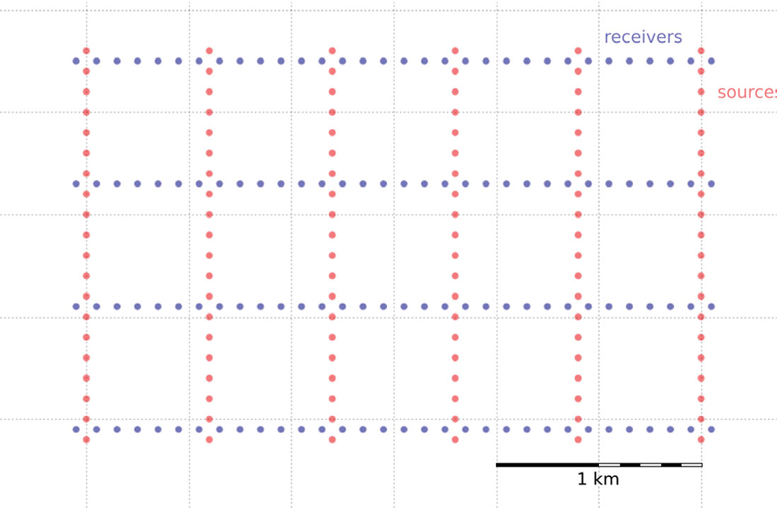
Plotting these lists is useful, but it is rather limited by itself. We’re probably going to want to do more calculations with these points – midpoints, azimuth distributions, and so on – and put these data on a real map. What we need is to insert these coordinates into a more flexible data structure that can hold additional information.

Making source and receiver points

Shapely is a Python library for creating and manipulating geometric objects like points, lines, and polygons. For example, Shapely can easily calculate the (x, y) coordinates halfway along a straight line between two points.

Pandas is a library that provides high-performance, easy-to-use data structures and data analysis tools, designed to make working with tabular data easy. The two primary data structures of Pandas are:

• Series – a one-dimensional labelled array capable of holding any data type (strings, integers, floating point numbers, lists, objects, etc.), and
• DataFrame – a two-dimensional labelled data structure where the columns can contain many different types of data. This is similar to the NumPy structured array but much easier to use.

GeoPandas combines the capabilities of Shapely and Pandas and greatly simplifies geospatial operations in Python, without the need for a spatial database. GeoDataFrames are a special type of DataFrame, specifically designed for holding geospatial data via a geometry column. One great thing about GeoDataFrame objects is that they have methods for saving data to shapefiles, which makes it easy to put our survey objects on a proper map.

Let’s make a set of (x, y) pairs for our receivers and sources, then we’ll turn them into Point objects, and add those to GeoDataFrame objects, which we can write out as shapefiles.

Arrange lists into x,y pairs with the zip function and create lists of Shapely Point objects:

rcvrs = [Point(x, y) for x, y in rcvrxy]
srcs = [Point(x, y) for x, y in srcxy]

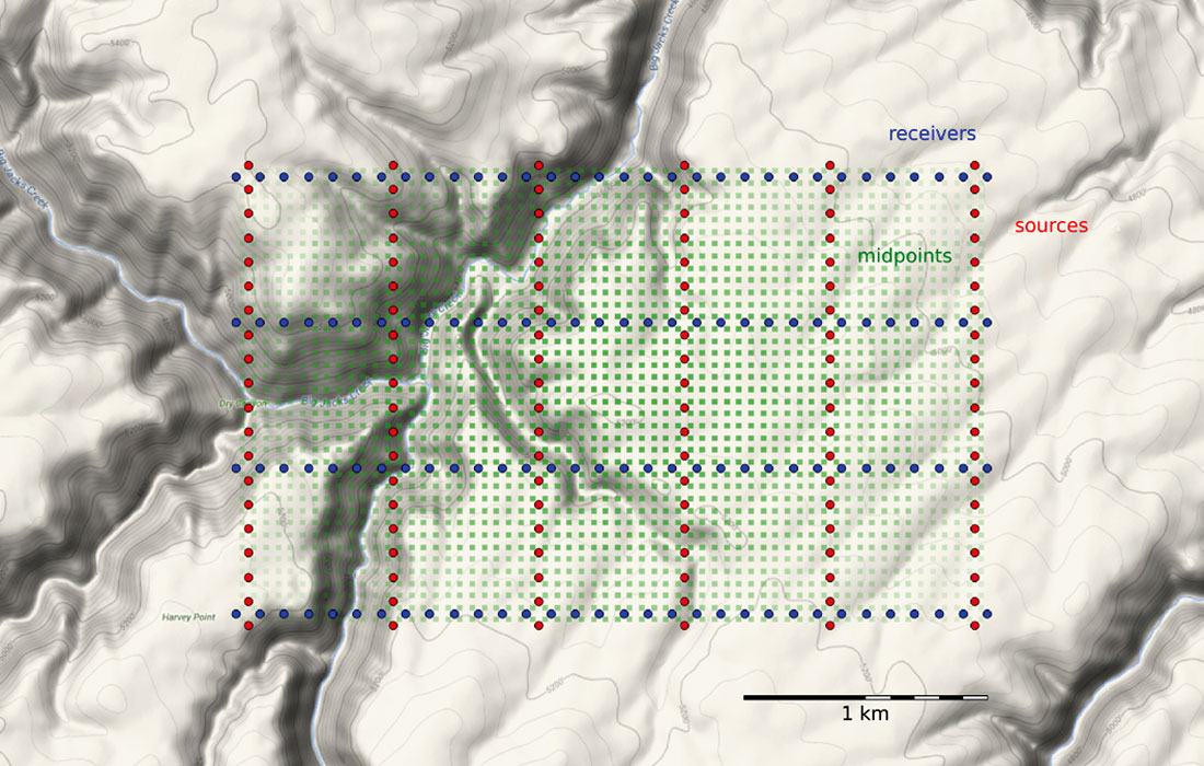
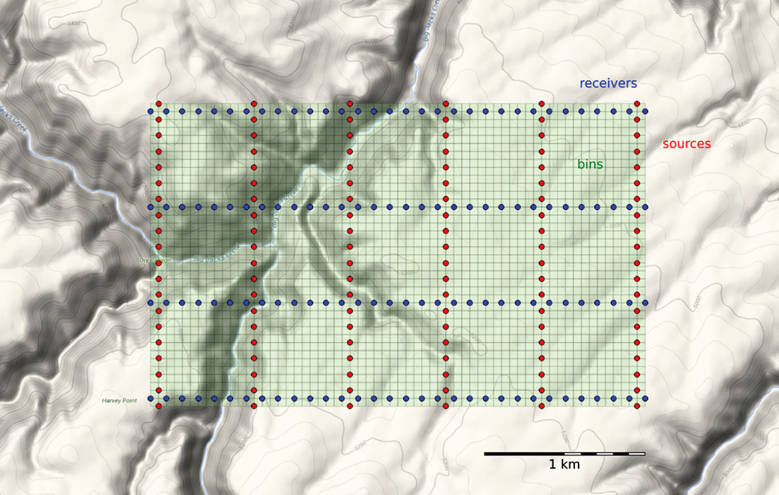
With our sources and receivers as a shapefile (see the accompanying IPython notebook for how to do this), it’s easy to import the survey into GIS software – we use QGIS – and layer it on top of a satellite image or physical topography map. For the purpose of this article, I’ve placed the survey in a bogus location riddled with canyons in southwestern Idaho, as shown in Figure 4.

Making midpoints

With sources and receivers as Shapely Point series, we can calculate a midpoint coordinate, offset distance, and azimuth for each sourcereceiver pair. The midpoint is found by creating a line segment (called a LineString in Shapely) starting from the source, ending at the receiver, and then interpolating the coordinate halfway along the line:

p = {'distanceˈ: 0.5, ˈnormalized': True}
midpoint_list = [LineString([r,s]).interpolate(**p)
   for r in rcvrs
   for s in srcs]

Shapely, a Point object has a method called distance for calculating how far it is to another point:

offsets = [r.distance(s)
   for r in rcvrs
   for s in srcs]

Some basic trigonometry yields the azimuth:

azimuths = [np.arctan((r.x - s.x)/(r.y - s.y))
   for r in rcvrs
   for s in srcs]

We combine these three series into a GeoDataFrame representing the midpoints of the traces in the survey. The midpoint_list is assigned to the geometry column of the GeoDataFrame, and we pass in the offsets and azimuths lists:

midpoints = geopandas.GeoDataFrame({
   'geometry': midpoint_list,
   'offset': offsets,
   'azimuth': np.degrees(azimuths) })

Making bins

Next we’d like to collect those midpoints into bins. We’ll use the so-called natural bins of this orthogonal survey – squares with sides half the source and receiver spacing.

Inlines and crosslines of a 3D seismic volume are like the rows and columns of the cells in your digital camera’s image sensor. Seismic bins are directly analogous to pixels – tile-like containers for digital information. The smaller the tiles, the higher the maximum realisable spatial resolution. A square survey with 4 million bins (or 4 megapixels) gives us 2000 inlines and 2000 crosslines of post-stack data. Small bins can mean high resolution, but just as with cameras, bin size is only one aspect of image quality.

Unlike your digital camera however, seismic surveys don’t come with a preset number of megapixels. There aren’t any bins until you form them. They are an abstraction.

Just as we represented the midpoints as a GeoSeries of Point objects, we will represent the bins with a GeoSeries of Polygon objects. GeoPandas provides the GeoSeries; Shapely provides the Polygon geometries. The steps are simple enough:

1. Compute the bin centre locations from the source and receiver locations using a nested loop.
2. Buffer the centres with a square. Normally buffers are circular, but we can use the lowest ‘resolution’ to get a square, and rotate it to align it with the survey.
3. Gather the buffered polygons into a GeoDataFrame.

The code, which you can read in the notebook, is unfortunately not very elegant. Better would be a method to generate a cartesian grid of quadrilaterals; we leave this as a challenge to the reader.

The green mesh in Figure 5 is the resulting map of polygons. These bins are what will hold the stacked traces after processing.

To create a common-midpoint gather for each bin, we need to grab all the traces whose midpoints fall within a particular bin. This is a sorting operation. And we’ll need to create gathers for every bin, which is a huge number of comparisons to make, even for a small survey such as this: 128 receivers and 120 sources make 15,360 midpoints. GeoPandas has a spatial join operation to index the midpoints into the bins:

reindexed = bins.reset_index()
   .rename(columns={ˈindexˈ: ˈbins_indexˈ})
joined = geopandas.tools.sjoin(reindexed, midpoints)

We originally performed this join with a nested loop – counting each midpoint into each bin with Shapely’s within function, removing midpoints as we went. This took about 30 minutes on an iMac. The spatial join operation, which uses highly optimized low-level libraries, takes 20 seconds.

The result is the old list of midpoints, but now with a new column indicating the index of the bin each midpoint belongs in. This makes it very easy to compute each bin’s statistics, using the Pandas groupby operation:

functions = {'fold': len, 'min_offset': np.min}
bin_stats = joined.groupby('bins_index')['offset']\
   .agg(functions)

It’s easy to add the statistics to the bin’s dataframe:

bins = geopandas.GeoDataFrame(bins.join(bin_stats))

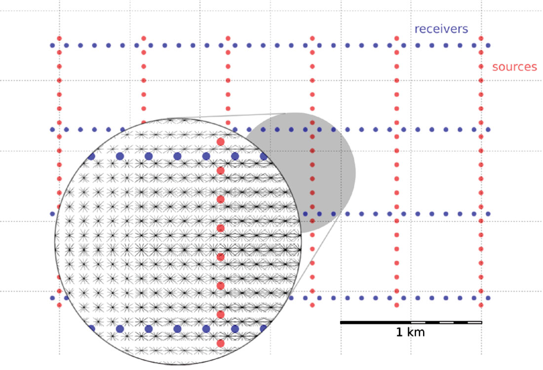
Now we can make displays of the bin statistics. Three common views are:

1. A spider plot showing offset vectors for each source-receiver pair at its midpoint location.
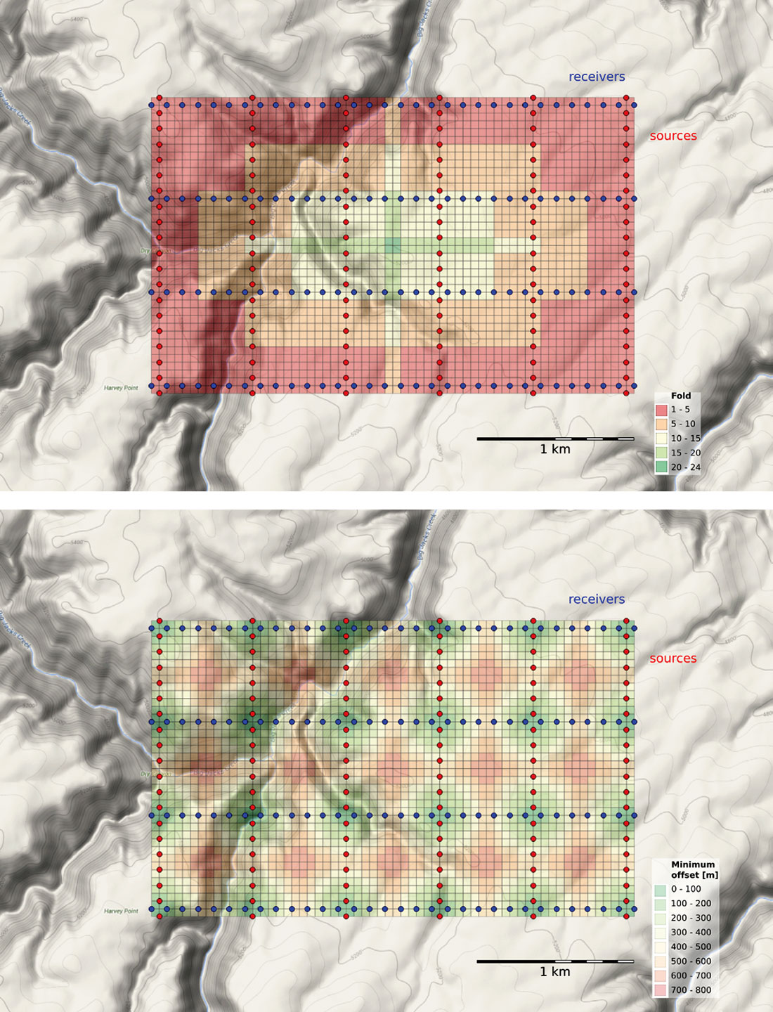
2. A fold map (the number of traces contributing to each bin).
3. A map of the minimum offset that is servicing each bin.

These maps are drawn using matplotlib, a 2D plotting library. For the offset and azimuth distribution in each bin, in Figure 6, we used quiver plots.

We use heatmaps to display fold and minimum offset statistics in the bins (Figure 7).

Making changes

So far, we’ve only created a theoretical survey. It has unrealistically uniform source and receiver locations, as if there were no surface constraints. It’s unlikely that we’ll be able to put sources and receivers in perfectly straight lines and at perfectly regular intervals. Topography, ground conditions, buildings, pipelines, and other surface factors have an impact on where stations can be placed. One of the jobs of the survey designer is to indicate how far sources and receivers can be skidded, or moved away from their theoretical locations before rejecting them entirely.

With 3D seismic data, the effect of station gaps or relocations won’t be as immediately obvious as a dead pixels on a digital camera, but they can cause some bins to have fewer traces than the idealized layout, which could be detrimental to the quality of imaging in that region. We can examine the impact of moving and removing stations on the data quality, by recomputing the bin statistics based on the new geometries, and comparing them to the statistics from the ideal spacing pattern.

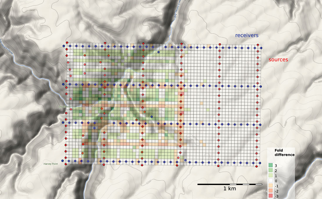
When one station needs to be adjusted, it may make sense to adjust several neighbouring points to compensate, or to add more somewhere nearby. But how can we tell what makes sense? The points should resemble the idealized fold and minimum offset statistics bin by bin. For example, let’s assume that we can’t put sources or receivers in river valleys and channels. Say they are too steep, or water would destroy the instrumentation, or are otherwise off limits. For source and receiver points located on steep canyon walls, or water courses, I used the graphical point editing tool in QGIS, to reposition these points to flatter, supposedly more accessible ground locations. The amended geometries are then sent back to Python for recalculating the survey statistics (Figure 8).

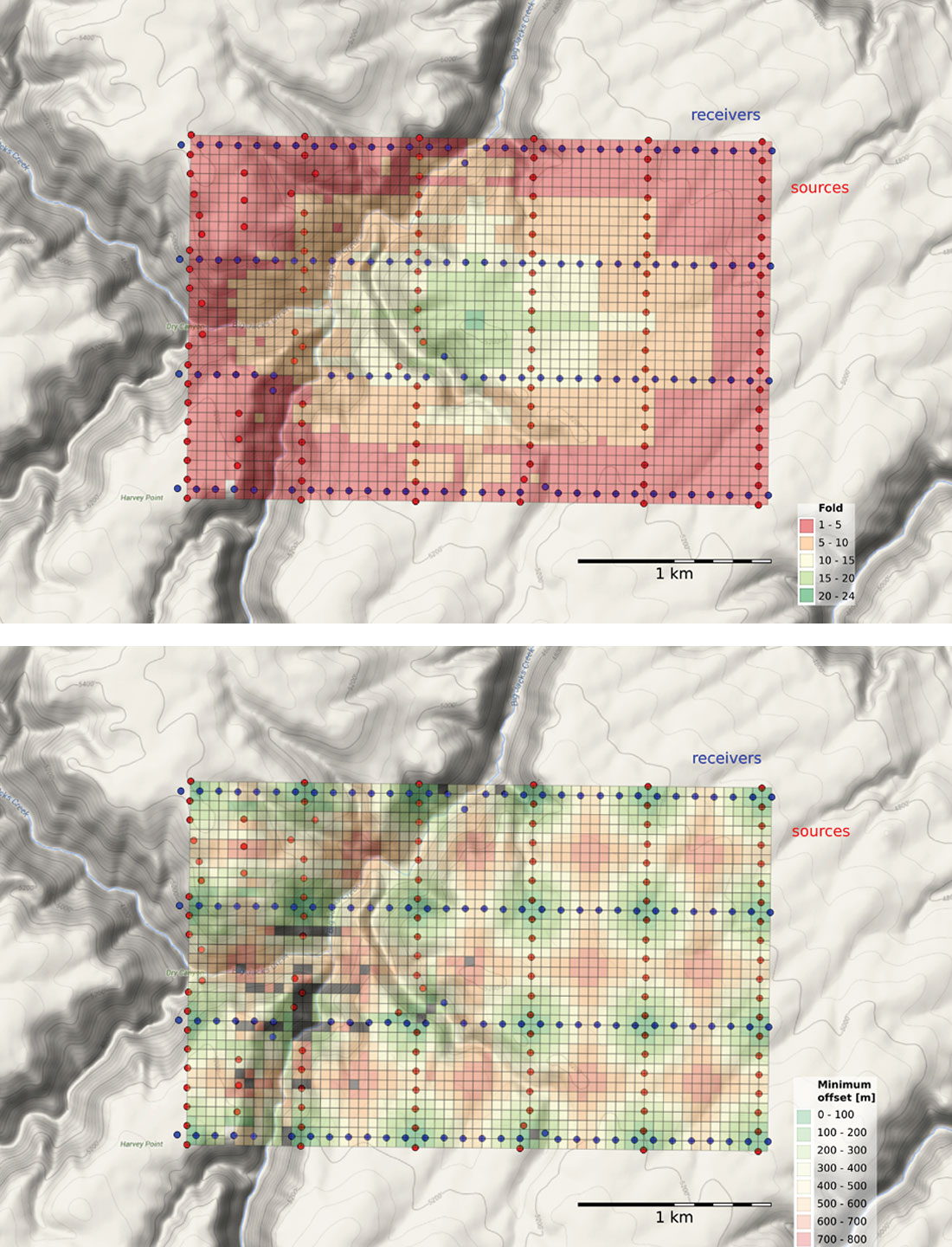
Bins that have a minimum offset greater than 800 m are highlighted in grey. These are the locations where we won’t expect to see the shallowest reflection (Figure 2). We can also calculate the difference between amended survey geometry and the idealized layout. Figure 9 shows the fold count has increased, decreased, or stayed the same as a result of our tweaking.

Summary

In this article, we’ve created a design for a 3D seismic land survey starting from a simple configuration of source and receiver surface coordinates. We organized and sorted the trace records from our would-be survey into bins, and we calculated a variety of bin statistics for mapping imaging quality indicators: offset distribution, azimuth distribution, fold, and minimum offset. Lastly, we changed the positions of a number of sources and receivers, and recalculated our survey statistics to highlight areas at risk of being underserved by insufficient sampling.

When experiments are cast into code, we can change the experiment by changing the code or in this case, changing the input parameters. As a result, the code becomes a powerful medium through which the geoscientist can ask questions of his or her data, and gain a deeper insight into the physical system.

Get the full code

The code used in this article is available as IPython notebook on GitHub at https://github.com/CSEG/Programming.