Preconditioning of Seismic Data Prior to Impedance Inversion

The calibration of seismic data with the available well control is an important step that provides the link between seismic reflections, their stratigraphic interpretation and subsequent prediction of reservoir and fluid properties. The standard practice to do this has been to produce synthetic seismograms from well logs with a bandwidth similar to that of the seismic data. The synthetic traces are produced by picking up the sonic and density logs for a well and calculating the reflection coefficients. These reflection coefficients are then convolved with a suitable zero or minimum phase wavelet and choosing a frequency response similar to that of seismic. The wavelet could also be extracted from the seismic data. Thereafter, the synthetic seismogram is displayed in the same polarity as the seismic and either overlaid or inter-fixed on the seismic data at the location of the well, after making a shift adjustment in time. Such a correlation helps to quickly identify individual reflections which can then be interpreted on the seismic data.

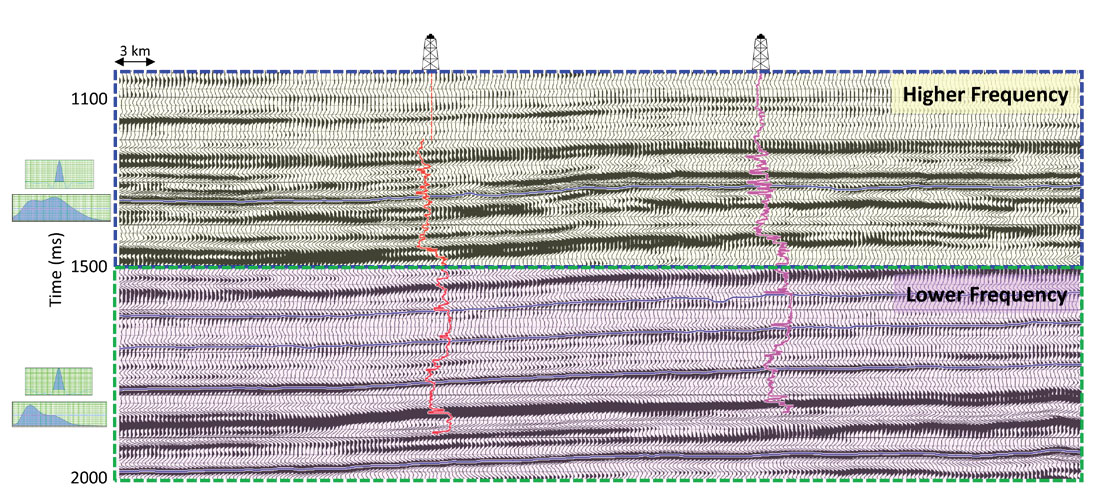
The frequency content of surface seismic data varies with time due to attenuation or other effects, so that generally we see higher frequencies in shallow intervals which are gradually lowered with increasing times. In Figure 1 we show a seismic section over a 1s interval, but higher frequencies in the upper 500ms and lower frequencies in the lower 500ms are seen. This can be seen on the wavelets that are extracted in the upper and lower intervals and the frequency spectra generated for the two intervals, as shown in the insets.

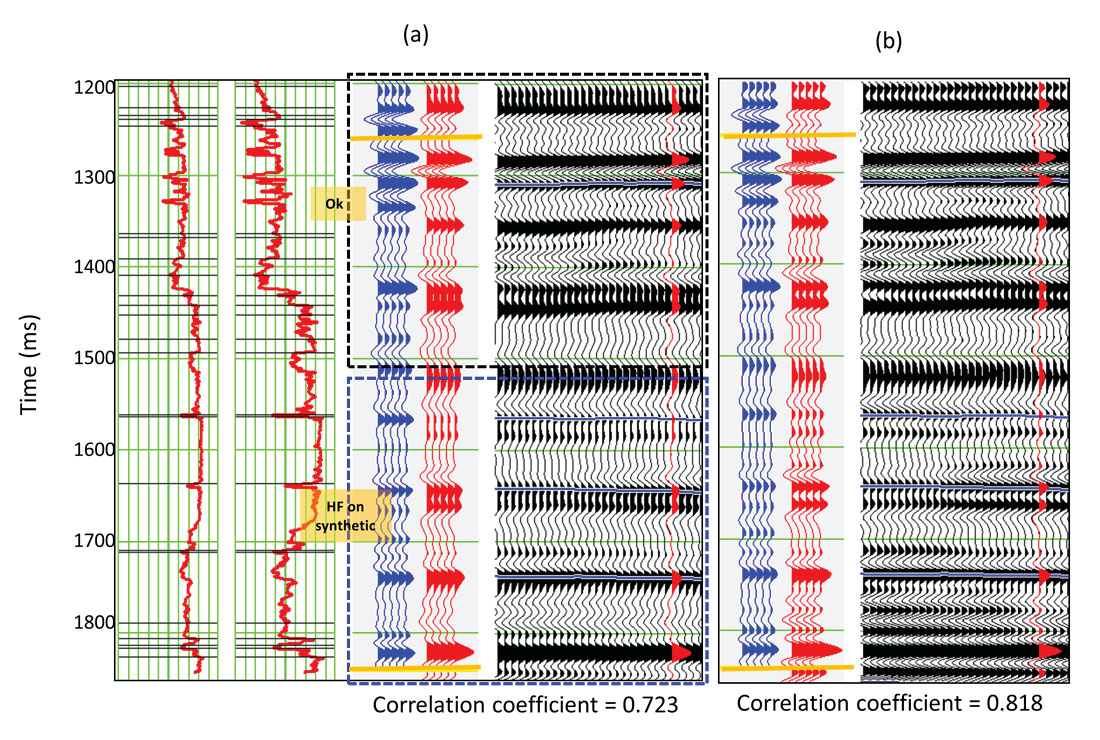
A synthetic seismogram generated using the wavelet from the shallower interval would exhibit a reasonable frequency match in the upper interval, but will show a higher frequency content for the lower interval as compared with the seismic data. We show this in Figure 2, where in (a) we have the P-velocity and density logs used for generating the synthetic traces in blue. These are compared with the real seismic traces in red, and the correlation coefficient between them is 0.723. Notice in the shallow portion highlighted with the black dashed box the frequency content between the synthetic and the real traces seems similar. However, in the deeper portion highlighted with the blued dashed box, the synthetic traces seem to exhibit a somewhat higher frequency (HF) content. As mentioned above, this is because the wavelet extracted from the upper interval was used for generating the synthetic seismogram.

One way to address this problem would be to extract an average wavelet over the full window and then generate a full-window synthetic seismogram that could be correlated with the seismic. However, this would have a lower resolution in the upper window and a higher resolution in the lower window, something that is contrary to what we expect.

Another way that could be adopted is that separate wavelets are extracted in the upper and the lower windows and separate synthetics are generated and compared. As well, the inversions would need to be performed in separate windows, which is time-consuming. In such an exercise, we can expect to see lower resolution in the lower window compared to the upper window.

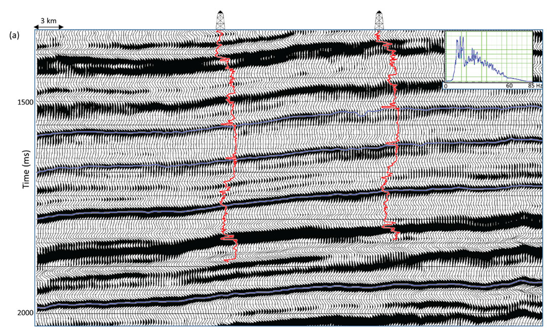
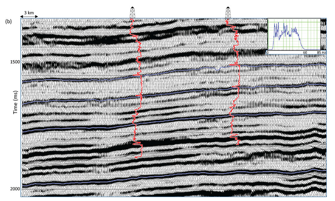
If we go back and examine the input seismic data we see that the bandwidth of the data is somewhat narrow, with the peak frequency at 12 or 15 Hz and noise after 60 Hz. Also, the frequency spectrum shows a roll-off after 30 Hz. In Figure 3a we show a segment of a seismic section from the input data, and the frequency spectrum is shown in the inset. To be able to extract some more information from the data, we should at least be able to make the frequency spectrum look flatter.

We achieve this with thin-bed reflectivity inversion, a process that extracts time-varying wavelets from the seismic data and using principles of spectral inversion produces sparse reflectivity estimates. The advantages include being able to pick up more reflection detail, to perform more accurate interpretation on seismic volumes obtained by convolving reflectivity volumes with wavelets of higher bandwidth than the input data, and to visualize subtle anomalies when some attributes are run on thin-bed reflectivity inversion output. More detail on this method and its applications can be picked up from the May 2008 and July 2009 issues of AAPG Geophysical Corner.

We put the input seismic data through thin-bed reflectivity inversion, and derive the reflectivity volume. In principle, once the reflectivity volume is derived from the seismic data, it is possible to filter it back to a frequency bandwidth higher than the input seismic data. But there are some seismic interpreters in our industry who are not comfortable with the idea of enhancing the bandwidth of the data beyond the recorded frequencies. Keeping that in mind here we filter the derived reflectivity volume to the same bandwidth as the input seismic data, i.e. 5-10-50-60 Hz. The seismic section equivalent to the section shown in Figure 3a is shown in Figure 3b. Notice the improvement in the resolution detail, which is also seen on the frequency spectrum shown in the inset. The amplitudes of the frequencies beyond 25 Hz have been enhanced so that the spectrum now looks flatter. The correlation with the impedance logs also looks much better. We show a section of the data after thin-bed reflectivity inversion in Figure 2b, where the synthetic seismogram generated from the well log data shows a better correlation with the seismic data. The correlation coefficient is now seen increased from 0.723 to 0.818.

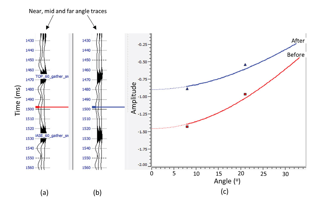
Usually a matter of concern for seismic interpreters is about the preservation of amplitude variation, both in the post-stack and the pre-stack seismic data. This is important for all AVO analysis work as well as impedance inversion performed on the seismic data. We picked up the pre-stack seismic data for a data volume from central Alberta, and after conditioning of the gathers, generated the near-, mid- and the far-angle stacks. This is the input required for simultaneous inversion which we have discussed earlier in our article published in the June 2015 issue of the AAPG Geophysical Corner. In Figure 4 we show the amplitude variation of the near-, mid- and far-angle traces for one such gather for two equivalent events, before and after thin-bed reflectivity inversion. We notice that though there is a small change in the amplitude of the events after thin-bed reflectivity inversion, which is expected, the relative amplitude variation with angle is very similar.

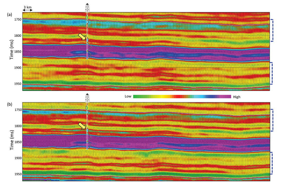
Finally, simultaneous inversion was run on the pre-stack data after preconditioning and thin-bed reflectivity inversion run on angle stacks. The result of the impedance inversion in the form of P-impedance sections, before and after thin-bed reflectivity inversion are shown in Figure 5a and b. The overlaid impedance logs are shown as curves as well as colored strip logs. Notice the mismatch indicated with the yellow arrow between the log and the inverted impedance values in Figure 5a, whereas it shows reasonably good match between the two in Figure 5b. Also, in the intervals indicated by the dashed blue braces to the right, many of the events are seen better well-defined and more focused in Figure 5b than Figure 5a.

We thus conclude from the above exercises that the varying frequency content in seismic data can pose problems while carrying out synthetic seismogram correlation to seismic data. The roll-offs that are seen on the frequency spectra of input seismic data can be flattened out with the application of thin-bed reflectivity inversion. This application is a post-stack process but can be fruitfully run on the near-, mid- and far-offset stacks, which can then be put through simultaneous impedance inversion. The results of such exercises can lead to more accurate interpretations which obviously help the bottom line.

Acknowledgements

We thank Arcis Seismic Solutions, TGS, for allowing us to present this work.