Pre-stack land surface and interbed demultiple methodology An Example from the Arabian Peninsula

Abstract

This case study shows the application of data-driven multiple removal techniques to a land data set from the Arabian Plate. Strong surface and internal reverberations are removed using a standardised processing flow, while preserving the original geometry for subsequent processing. This paper highlights some of the practical aspects of applying these techniques in the production processing of land seismic data.

Introduction

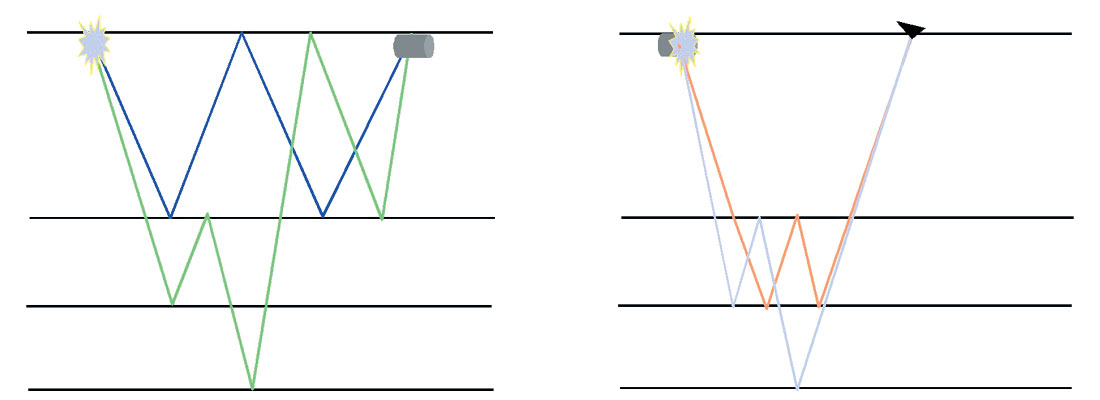
On land, strong surface multiples can contaminate the data when the near surface layer is consolidated and a strong surface reflector is present. In most land cases there is not a sufficient difference between primary and multiple stacking velocities and thus multiple and primary reflected energy have similar moveout characteristics. Demultiple technologies; such as Radon application (and its enhanced versions) based on velocity discrimination and consequently curvature differentiation are likely to fail. In addition, long period surface multiples are often present which makes demultiple methods based on predictive deconvolution (either in t-x or t-p) not always the optimal solution. Data-driven multiple removal methods like Surface- Related Multiple Elimination (SRME) and Interbed Multiple Elimination (IME) have proven to be valuable tools to remove multiples (surface and interbed) without using any type of a priori information about the subsurface. Figure 1, shows the types of multiple handled by:

(a) SRME – All surface multiples

(b) IME – interbed multiples.

However, because these techniques employ the recorded data in order to predict and then subtract the multiples, the pre-conditioning of the input data is paramount to the successful application of the method. In comparison with marine data, land datasets often exhibit highly irregular geometries, complex azimuthal distributions and poor signal-to-noise ratios.

Pre-processing and fourier regularisation

There are several pre-processing stages regarding the application of demultiple technologies to land data. Some of the major pre-processing steps are summarized below:

Pre-processing steps

• Application of field statics, and residual statics corrections
• Ground roll suppression (using f-k or optimised Radon filtering)
• Removal of spurious events, noise bursts etc.
• Infill of missing shots/receivers
• Trace balancing to obtain laterally consistent amplitude behaviour
• Filtering of data to remove spatial & temporal aliasing
• Amplitude recovery to turn 3D into 2D amplitudes

Note that there is a concentrated effort to correct for field and residual statics and to enhance the signal to noise ratio as this is critical to both wavefield regularisation and multiple prediction.

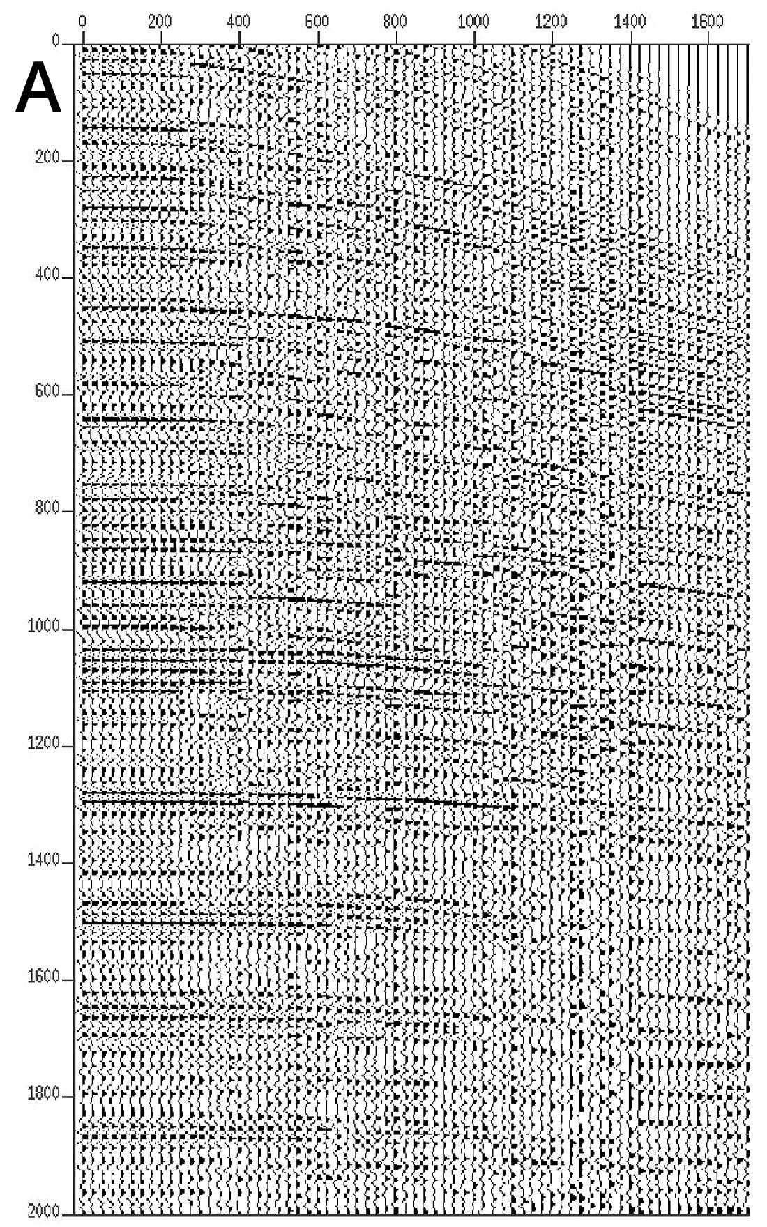
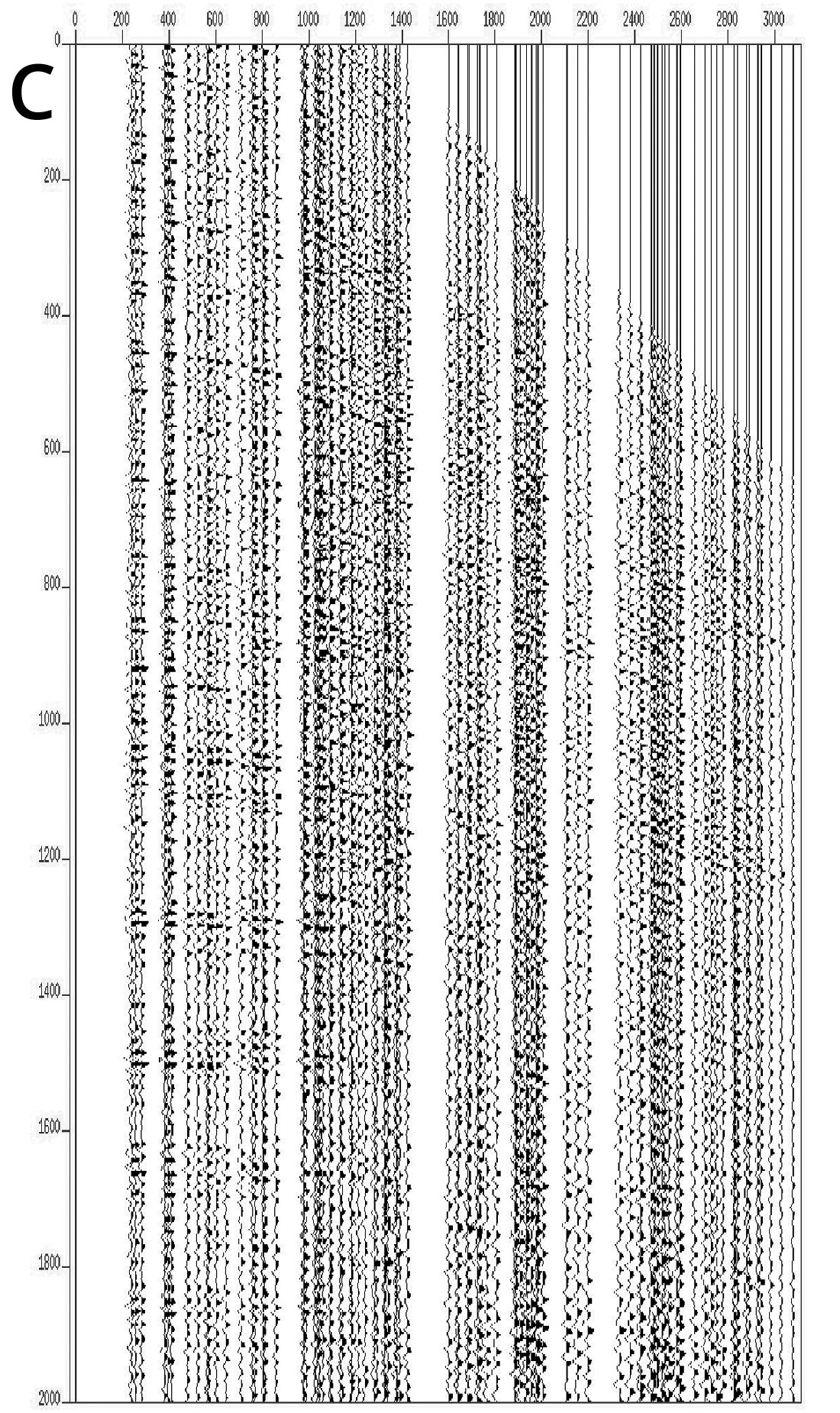
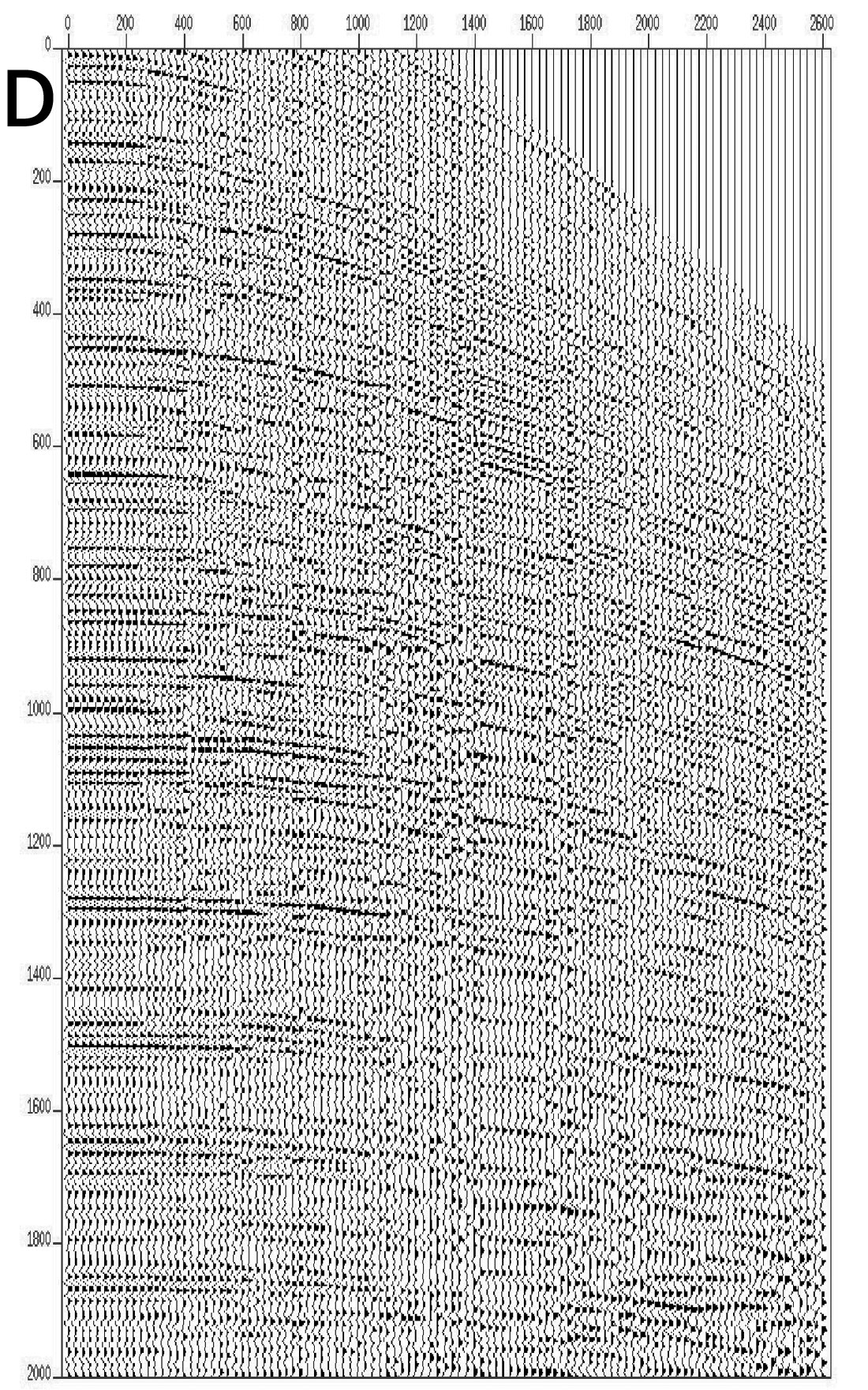
Following the pre-processing phase the next step is to apply wavefield regularisation. In practice we use the method of Fourier regularisation (Duijndam et al., 1999) where irregularly sampled data can be put on any desired regular grid, as long as they are spatially band limited. Fourier regularisation uses a least squares estimation of the Fourier spectrum from irregularly sampled data. Once the Fourier spectrum has been estimated, a standard inverse Fourier transform can be used to obtain the data on a regular grid (in the spatial domain). The method takes into account the exact spatial positions, does not use a geophysical model concerning the data or subsurface, and preserves amplitudes. Note that the regularised data are only used to predict multiples, and that the original geometry of the data from which the multiples will be subtracted remains unaffected. Figures 2a and 2b show a typical CDPgather before and after NMO applied. Note the irregular offset distribution and the lack of zero offset traces. Figure 2c, illustrates the same CDP gather with NMO applied, regularised and with zero offset extrapolated traces, whereas, Figure 2d, depicts the final regularized CDP gather after NMO removal. Note the continuity and uniformity of the seismic character with offset.

Surface and interbed multiple elimination

In surface related multiple elimination (SRME), the multiple-contaminated data is used as an estimate of the multiple-free data. After a 2D convolution of the multiple-contaminated data with itself, the predicted surface multiples are subtracted from the measured multiple-contaminated data in an adaptive way. For each user-defined window in time and space, a temporal filter is computed such that after convolution of this filter with the predicted multiples and subtraction of this result from the multiple-contaminated input data, a minimum energy is obtained. Considerable care must be taken in choosing the filter length and the window size. If the filter length is too long, it is possible to remove primaries, whereas if it is too short, it may lead to violation of the minimum energy criterion when primaries and multiple are interfering. However, a properly designed adaptive subtraction process should lead to good primary amplitude preservation.

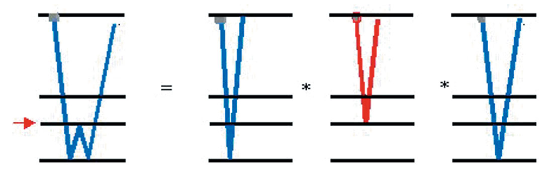
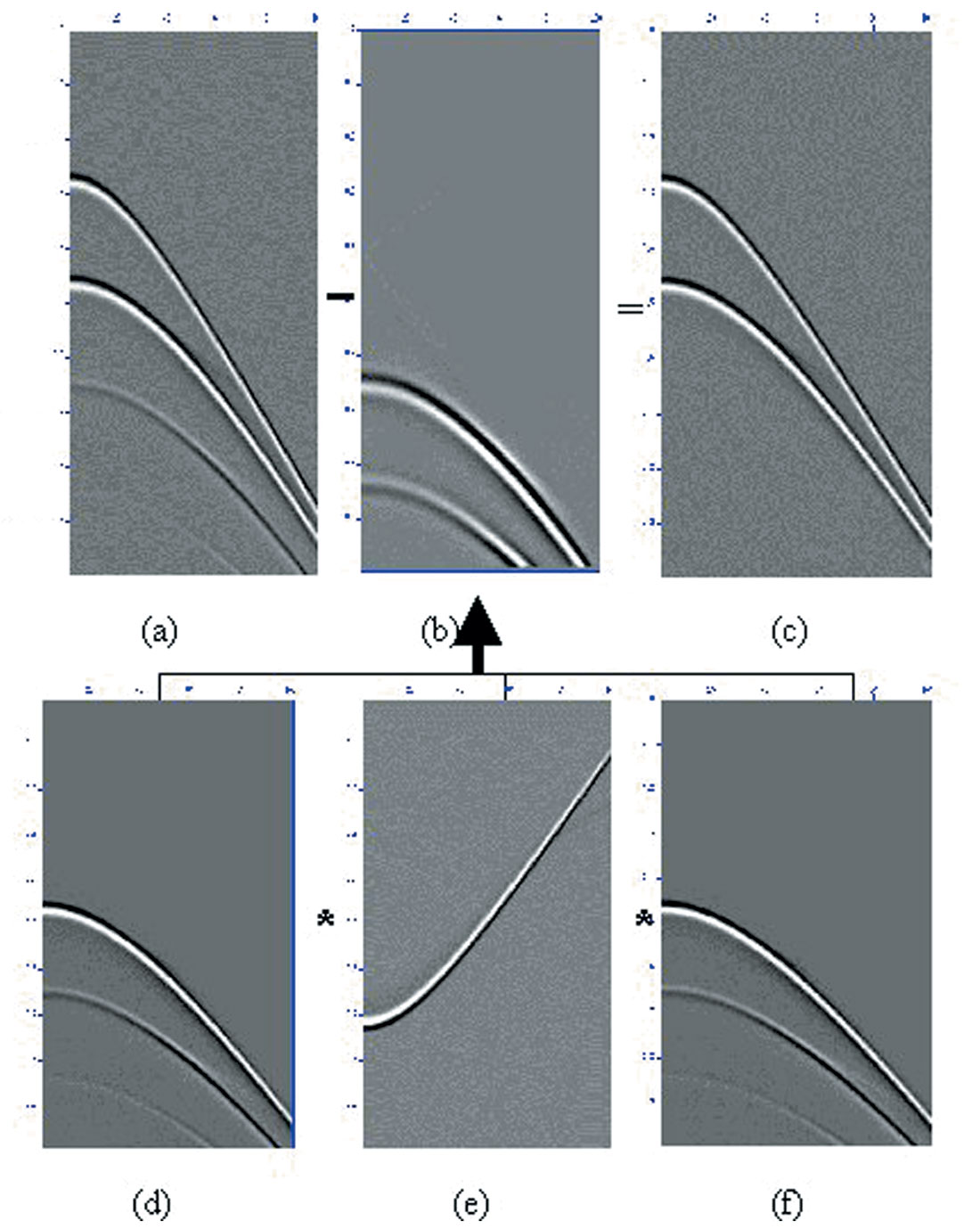
There are two common implementations of interbed multiple elimination (IME). Figures 3 and 4 illustrate the concept of boundary-related interbed multiple prediction, where interbed multiples generated by an identified (picked during interpretation) boundary are predicted. This procedure requires the multiple generator to be picked before the interbed multiple prediction can proceed. Figure 4a, illustrates the input gather with primaries and interbed multiples. Figure 4b, depicts the predicted interbed multiple model assuming a boundary as shown in Figure 3. This section is obtained by a double 2D convolution (ie: in time and space) comprised of the muted gather above, ie: without the primary P1, see Figures 4d and 4f, and the reverse gather muted below the P1 primary (Figure 4e). Figure 4c, is the resultant primaries only section after an adaptive subtraction of the input gather (Figure 4a) with the interbed multiple model (Figure 4b).

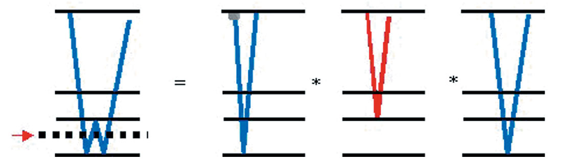
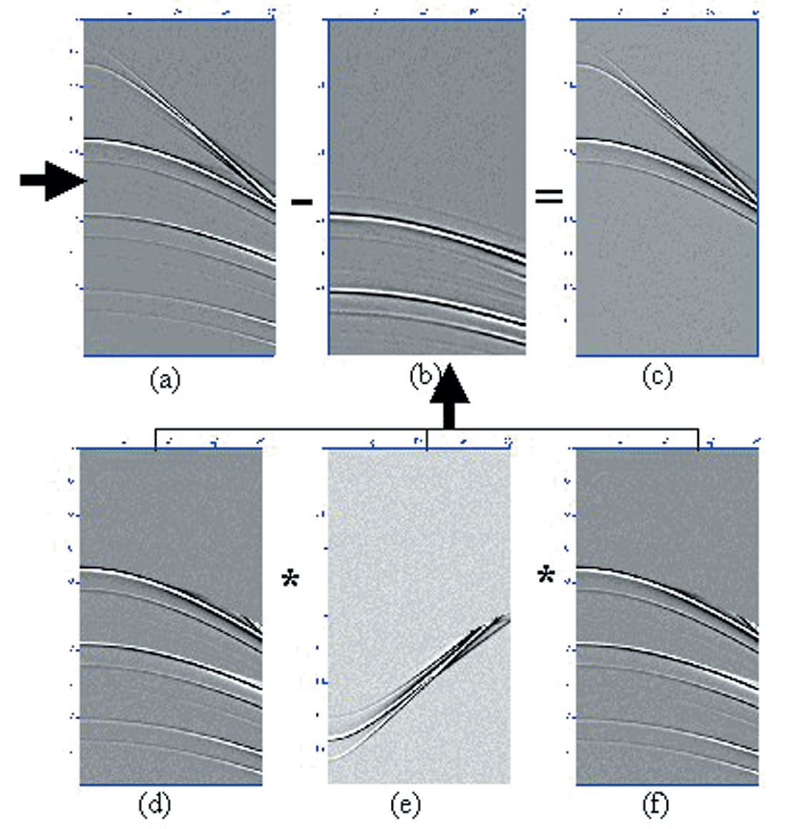
A second approach to remove interbed multiples is to assume a particular ‘pseudo boundary’ interface which does not necessarily have to follow a strong reflector (see Figures 5 and 6). The obvious advantage of this last approach is that less effort is required to pick such a ‘pseudo boundary’ as it may be a smoothed horizon between two strong reflectors, or even flat. The procedure to compute the interbed multiple model and the final primaries only section is similar to the one outlined in the previous paragraph, with the only exception that muting needs to be performed at the level of the ‘pseudo boundary’ interface (see Figures 5 and Figures 6a-6f).

Data example

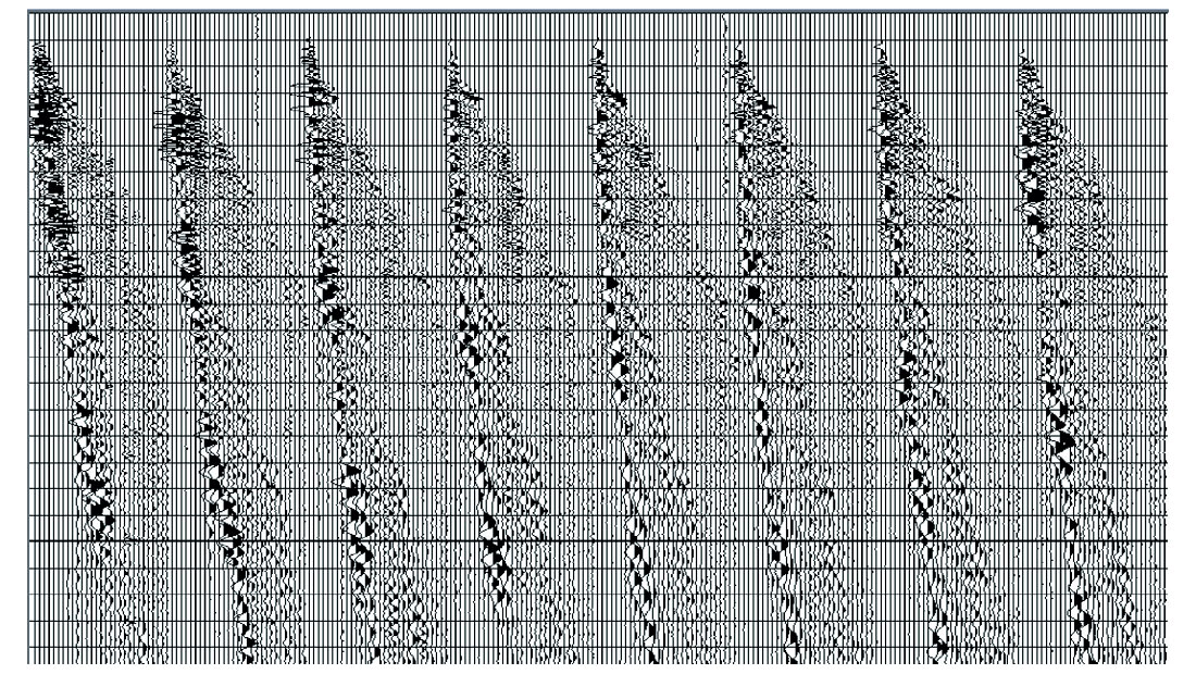
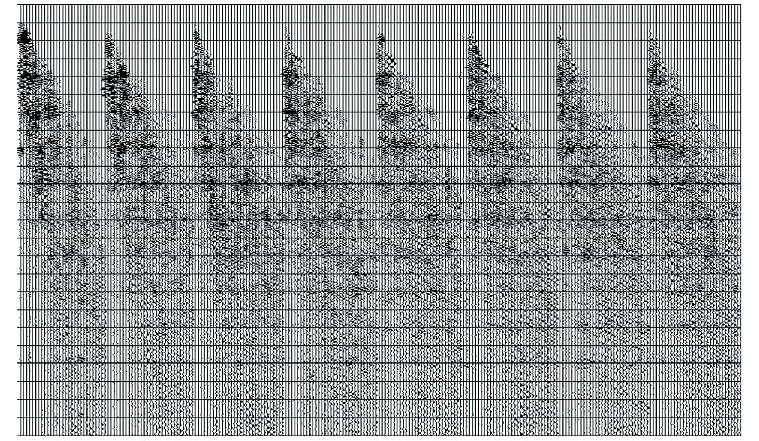
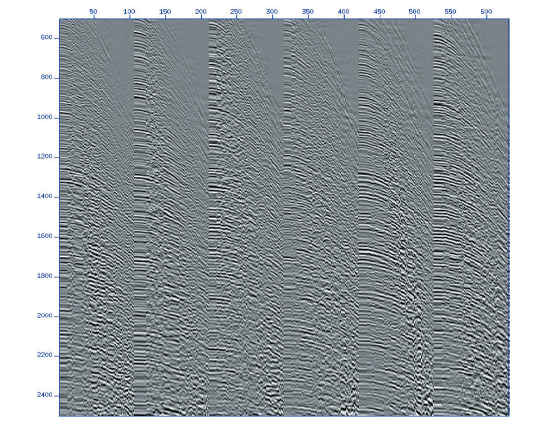
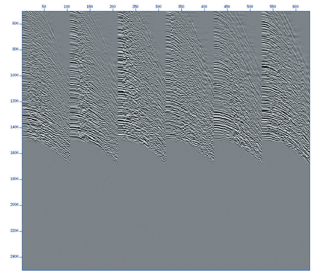
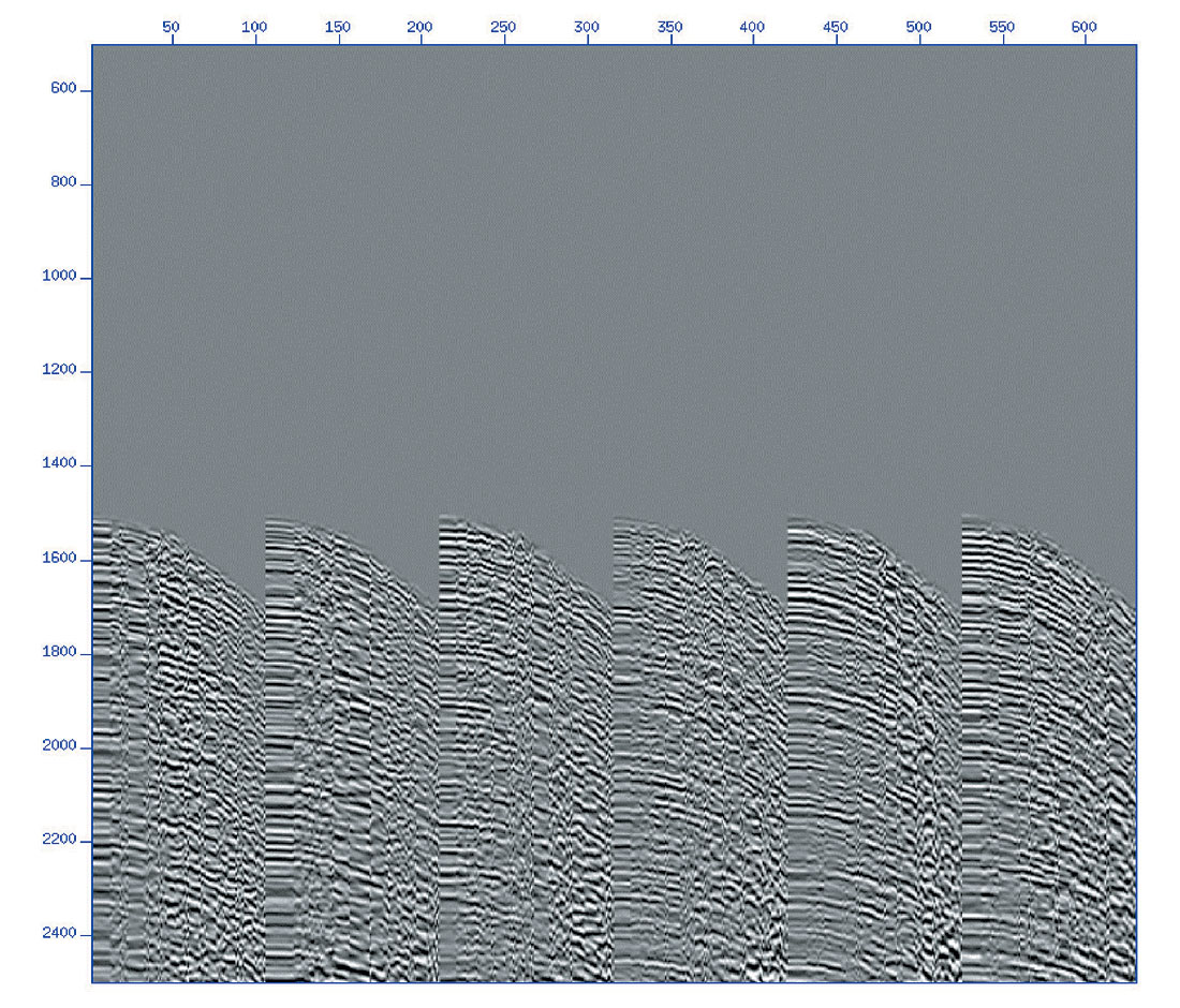
For these data from the Arabian Peninsula, the pre-processing sequence consisted of application of statics, ground roll removal by f-k filter, and a noise burst removal. The data were contaminated by short noise bursts, of unknown origin, at sporadic times down the record and in random locations. To remove this noise, sub spectral balancing was applied to the data using sample-wise median thresholding within frequency sub-bands in time-frequency space. Figures 7a and 7b show examples of several CDP gathers, before and after pre - processing and noise elimination applied, respectively. The data were then binned to the 3d processing grid and CDPs were gathered into super CDPs (SCDP) to decrease the offset spacing and further enhance the signal to noise ratio. Next, Fourier regularisation was applied in order to regularise the offset distribution within the obtained SCDPs and thus allow the use of SRME processing within each SCDP gather. The advantage of using this technique is that no a priori information is needed with respect to the subsurface during wave field regularisation. The only assumption made is that the data in the transform domain are band-limited. NMO and inverse NMO were wrapped a round the regularisation process to prevent spatial aliasing of events with large moveout. It should be noted that the regularisation itself helps to improve the signal to noise ratio since in the Fourier domain, the random components are not band-limited and will therefore not be reconstructed. In addition, Fourier regularisation allows the user to output data traces at any chosen grid spacing, thus it is possible to select an output trace distribution optimum for the SRME processing. A selection of SCDP gathers is depicted in Figure 8 (a). Figure 8 (b) shows the predicted free-surface multiples on SCDP gathers. After the prediction of the free-surface multiples, the next stage is the adaptive subtraction of the predicted multiples.

The following options exist: 1) restore the original geometry to the predicted multiples by inverse regularisation, and apply the adaptive subtraction from the original (non-regular) data in CDP domain or in the SCDP, or 2) apply the adaptive subtraction in the regularised domain, create a difference section to obtain the subtracted multiples, de-regularise the result, and subtract it from the original data (Kelamis and Verschuur, 2000). The inverse regularisation is applied to restore the data back to the original trace positions. However, for this data option 2 was found to work slightly better because of the dense spatial sampling after regularisation. It is well known that the performance of the adaptive subtraction filter depends on the spatial distribution of the traces in the input ensemble. Moreover, azimuth information is preserved because the predicted multiples are always subtracted from the original data.

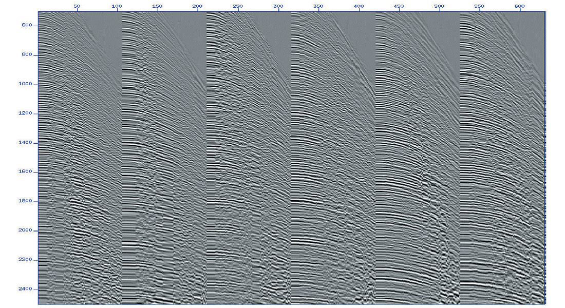
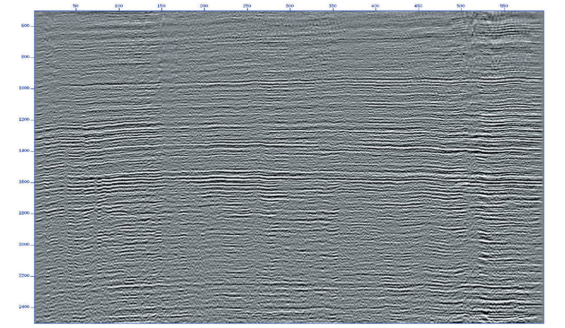
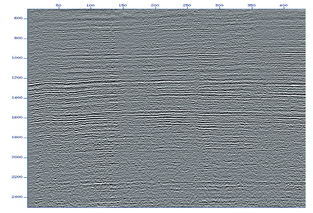
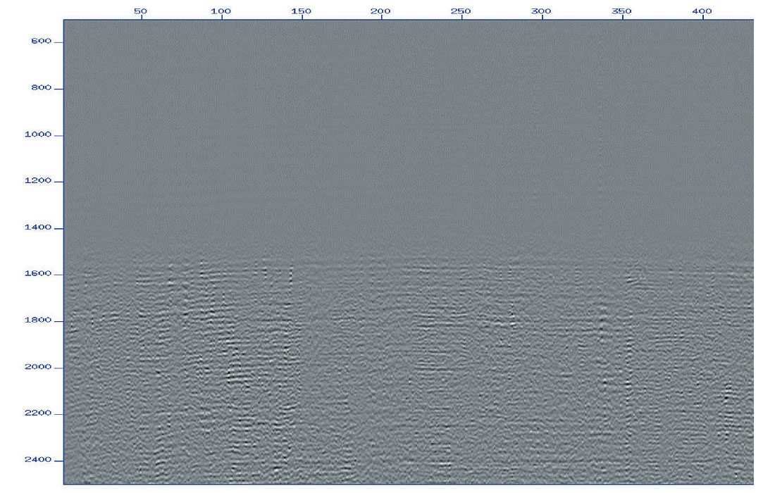
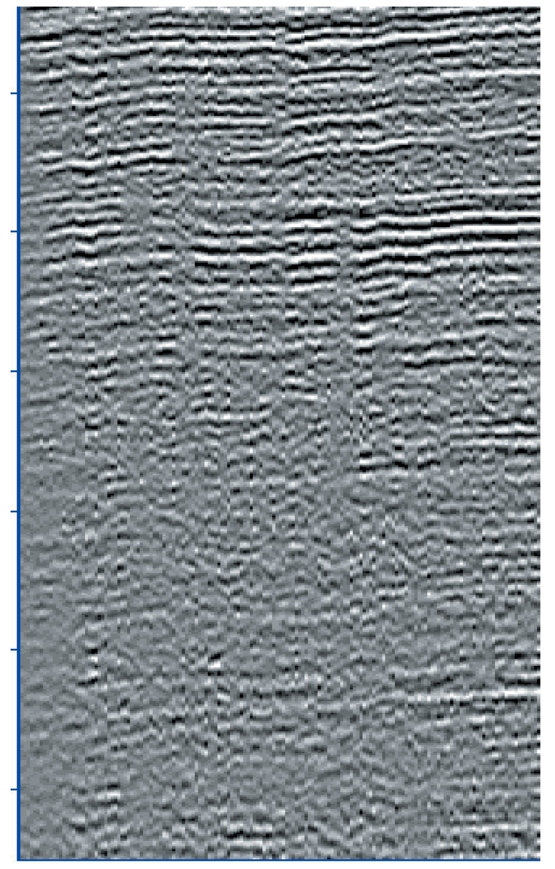
The corresponding stack sections namely, with and without free surface multiples are depicted in Figures 9(a) and 9(b), respectively. Figure 9(c) depicts the difference of the stack before and after the SRME application. A substantial reduction of surface multiple reverberations can be observed.

When the surface related multiples have been attenuated the interbed multiples now stand out. The removal or attenuation of the interbed multiples can be addressed by an SRME related technique proposed by Jakubowicz (1998) and illustrated by Van Borselen (2002). The approach requires only the identification (i.e. picking) of the multiple generator(s), or alternatively, a ‘pseudo-boundary’ across which interbed multiples have propagated. Then, through a double convolution of appropriate gathers, internal multiples can be predicted followed by an adaptive subtraction step, similar to the one performed during the SRME application. The optimised processing strategy leads to efficient removal of either interbed multiples that are generated by a (chosen) internal reflector, or interbed multiples that have crossed a (chosen) pseudo boundary during wavefield propagation.

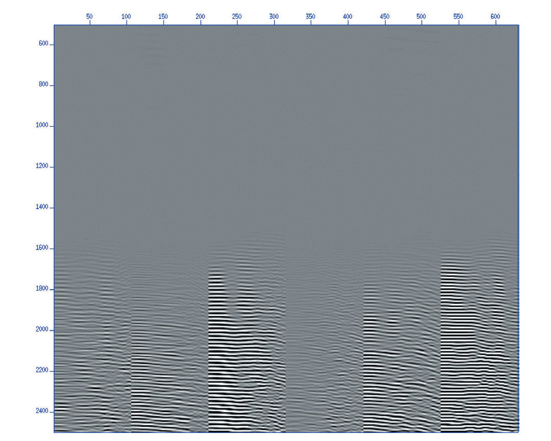
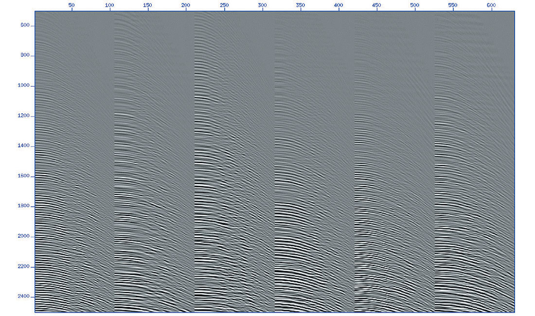
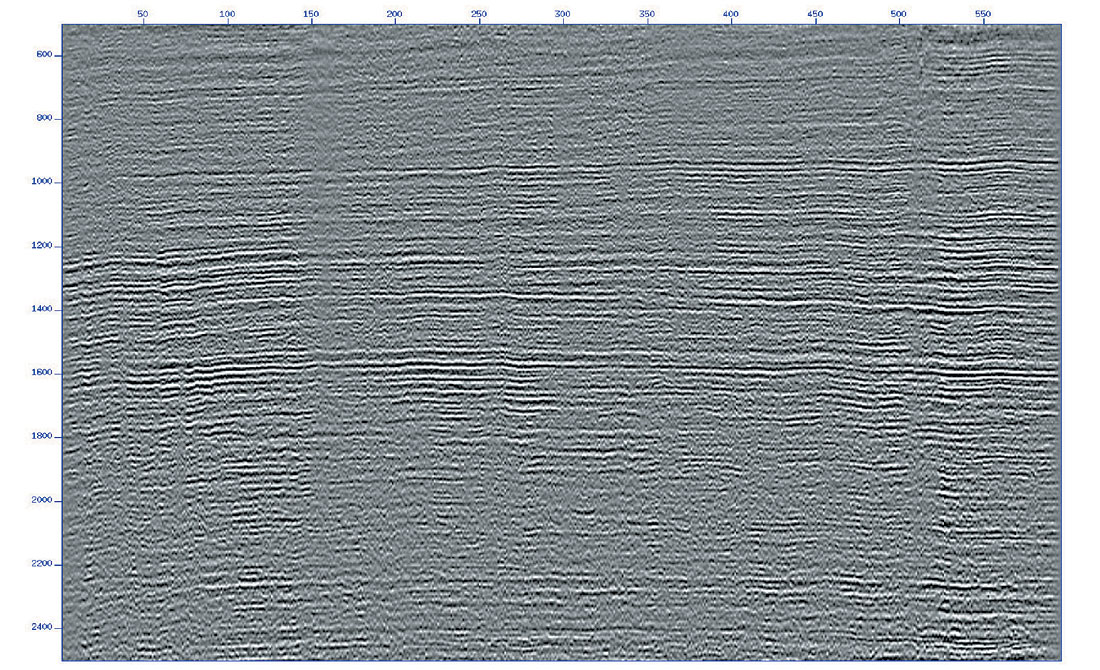
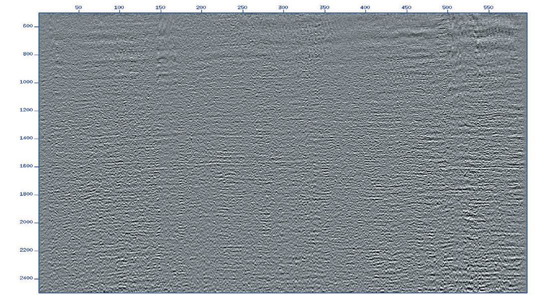
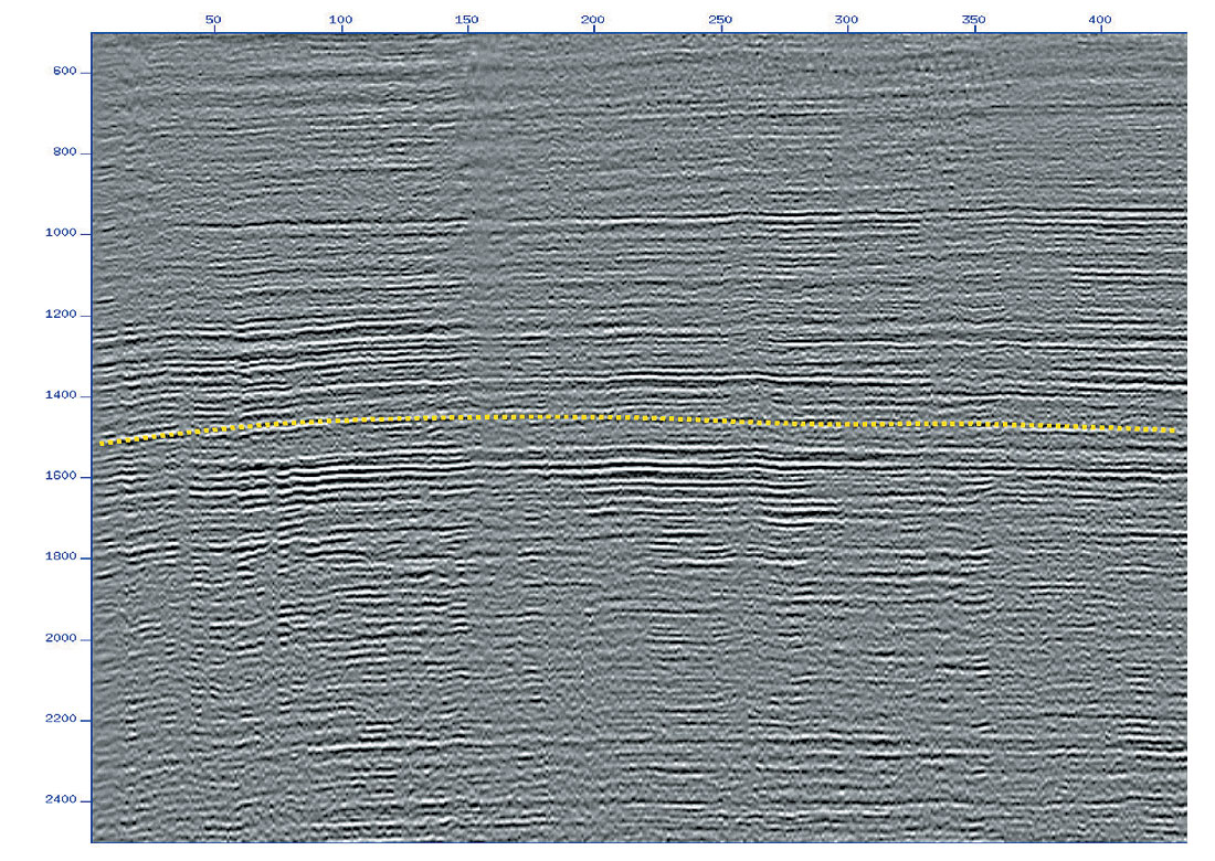
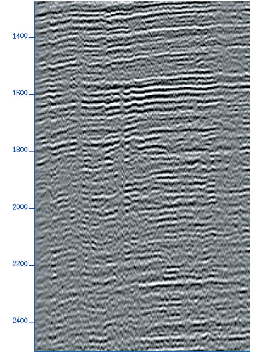
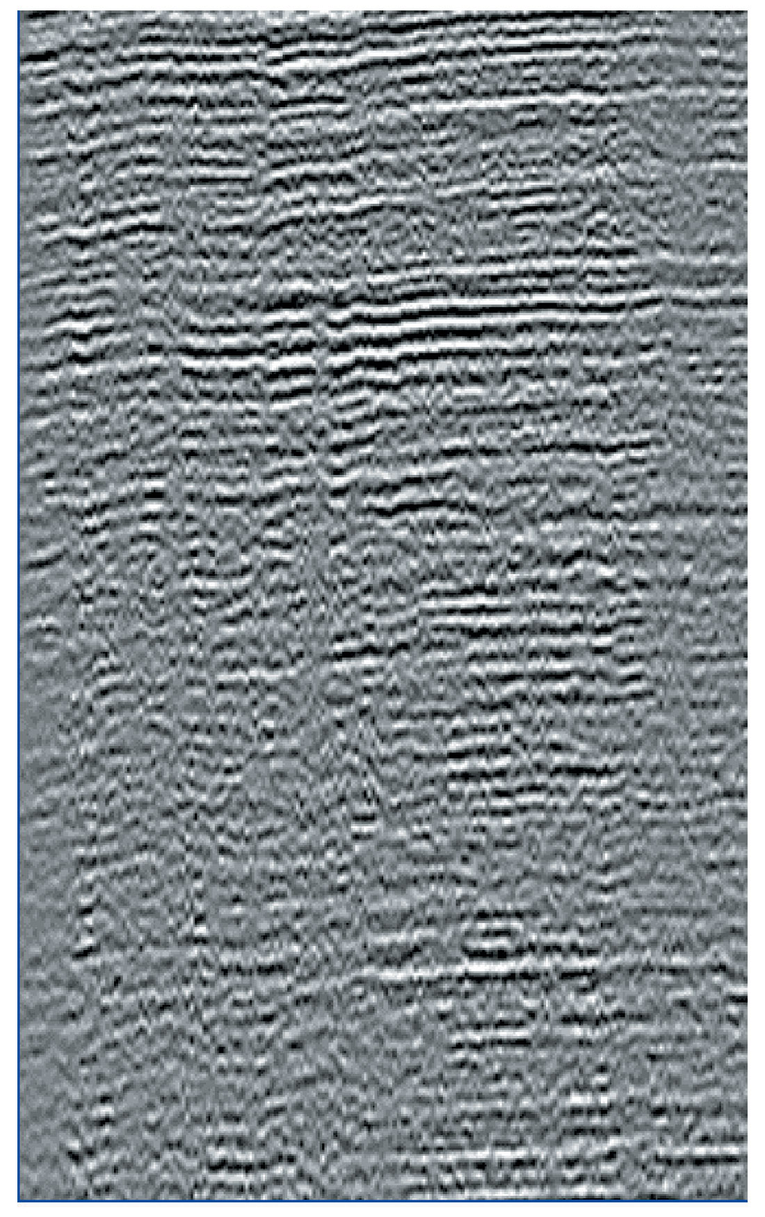
For this case study, it was deemed best to process the data using the later approach since the location of the main interbed generators were unclear. A Fourier regularisation step was also necessary during the application of Interbed Multiple Elimination (IME). After the identification of the pseudo-boundary, as depicted by the yellow line on Figure 11(a) above the target horizon, IME was run on the regularised SCDPs. Figures 10a-c show the input and muted SCDP gathers, respectively during the interbed multiple prediction stages. Figure 10(d) shows the SCDP gathers exhibiting the predicted interbed multiples derived for the assumed pseudo boundary. To preserve geometry and maintain all azimuthal information, the predicted multiples are ‘de-regularised’ before the adaptive subtraction from the original (irregular) data. Figures 11(a) shows a stack of the pre-processed input data (same as Figure 9(a)). Figure 11(b) shows the stacked results after the application of SRME and IME with the pseudo boundary method as depicted with the yellow line shown in Figure 11a. Figure 11(c) illustrates the difference of the two sections. Figures 12 a, b and c are detailed sections which clearly illustrate the differences and the added value to the interpretation of the free surface and interbed multiple removal processes. Note the significant additional reduction of internal reverberations in the data.

Conclusions

In situations during land data processing, where the primary and the multiple stacking velocities exhibit similar moveout characteristics, data-driven multiple removal techniques, such as SRME and IME, can be effectively applied in order to reduce surface and interbed multiple contamination and consequently enhance seismic interpretation. The main pre-processing steps include removal of spurious events and surface waves, surface consistent amplitude balancing and residual statics corrections. In addition, the use of Fourier regularisation and inverse regularisation on the multiple model estimates allows an effective adaptive subtraction and the preservation of geometry configuration for subsequent processing.

Acknowledgements

The authors thank ADCO and ADNOC for permission to show their data and PGS Geophysical for permission to publish this paper.