Introduction
This article is the second of two parts following part 1 in the March 2006 RECORDER.
Part 1 described the potential of conventional isotropic AVO to identify optimum geo-mechanical properties for the successful exploitation of tight gas shale Resource Plays through effective hydraulic fracture stimulation. Based on comparisons to the Barnett shale, the optimum gas shale properties have relatively low λ’s (incompressibility) and high µ’s (rigidity) that give rise to geo-mechanical brittleness capable of supporting extensive induced fractures. Furthermore these properties also produce the lowest closure stresses (i.e. largest fractures) due to the λ/(λ+2µ) ratio term in the closure stress equation.
The isotropic AVO modeling based on log and core analysis tied to 3D data indicated that shale zones with properties that best matched the Barnett shale analogue, had mostly type 1 AVO responses i.e. high P-wave and shear-wave impedances relative to background.
Part 2 of this article will investigate the potential of AVO variation with azimuth (AVAZ) to detect anisotropy due to natural fractures or in-situ stress, that would ideally corroborate the mapping of optimal fracture prone zones from the isotropic AVO in part 1. The high impedance model values established in part 1, will be the basis for the AVAZ analysis described below.
Examples of Azimuthal AVO
The literature abounds with numerous excellent examples and observations of AVAZ some of which are shown here in order to better understand the expectation and potential in pursuing this type of analysis (Lynn et al., 1996, 2004, Gray et al., 2000, 2002, Williams and Jenner 2002, Neves et al., 2003 and Todorvic-Marinic et al., 2005). For a comprehensive review and explanation of recent technical advances, I recommend Heloise Lynn’s fall 2004 SEG/AAPG Distinguished Lecture (TLE 2004) and webcast that is accessible through the CSEG website.
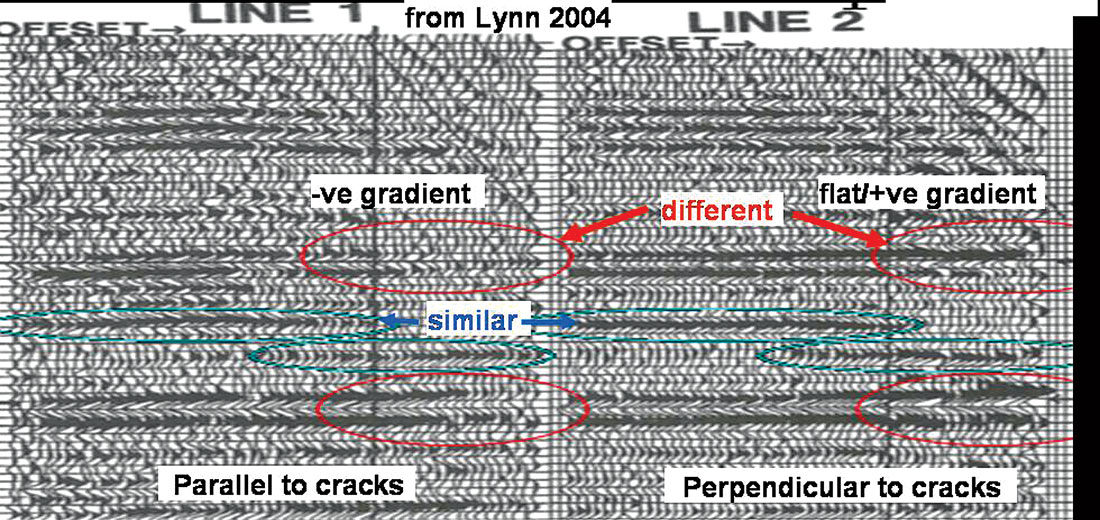
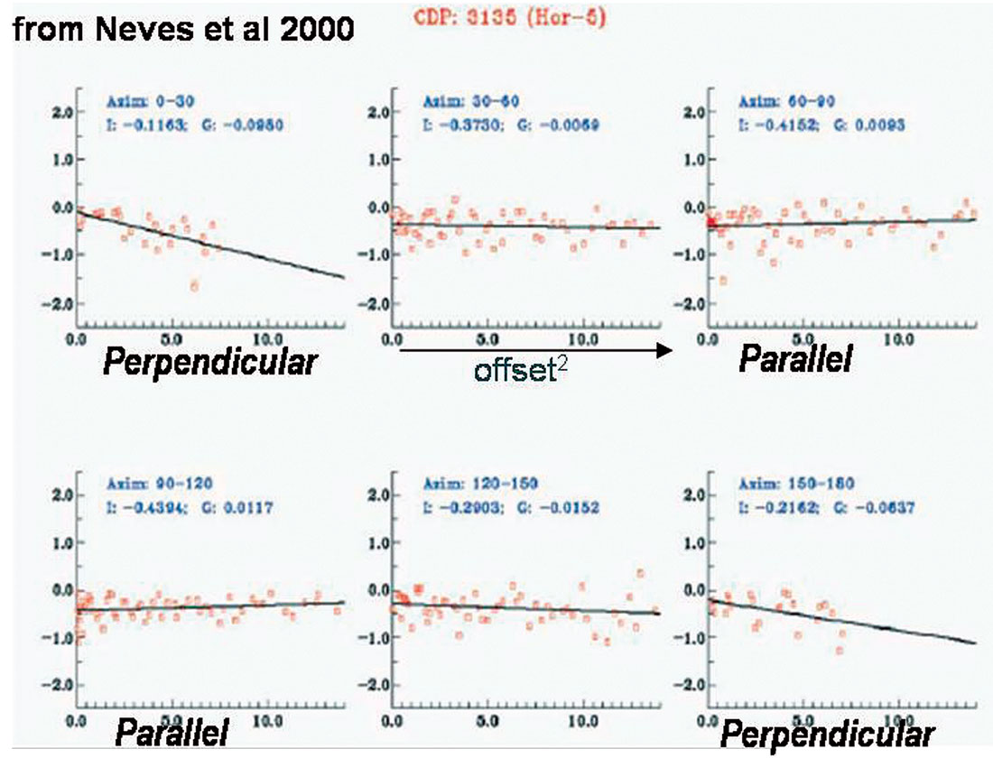
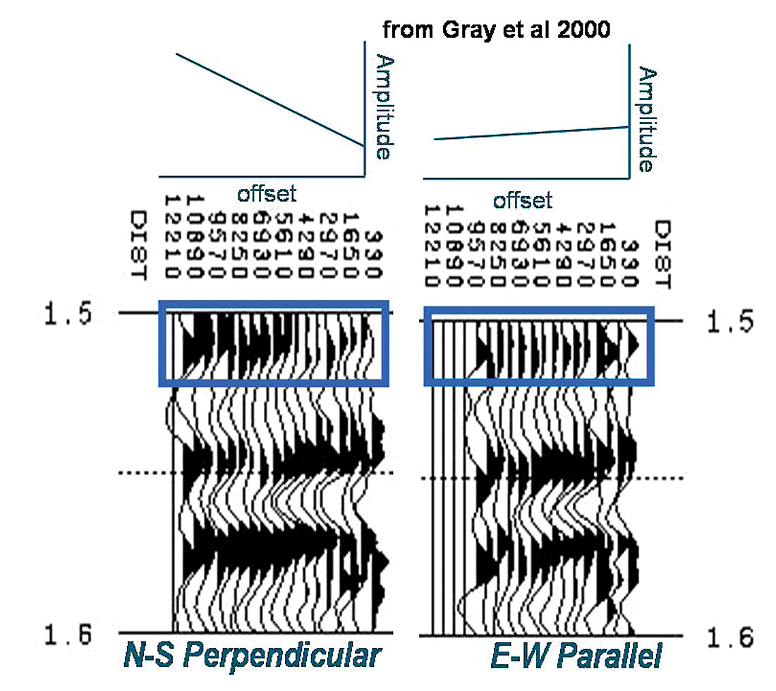
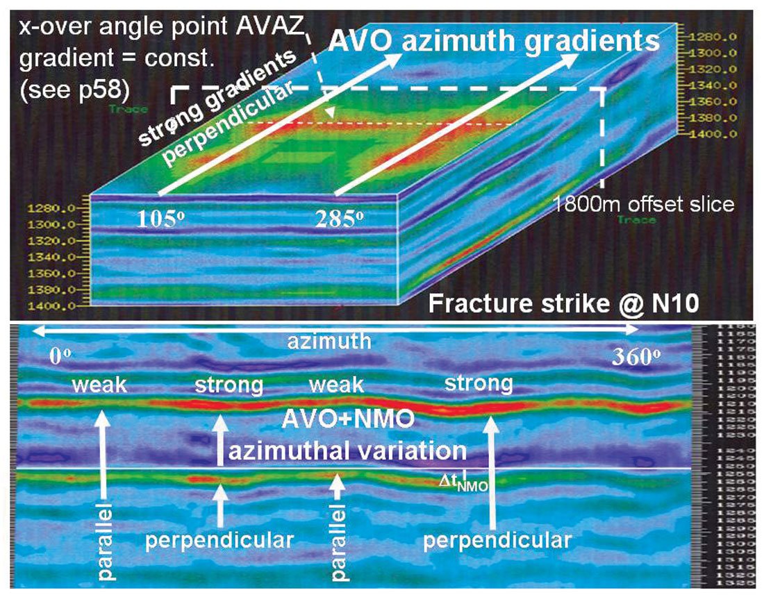
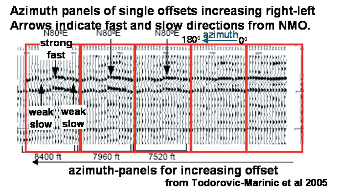
Figures 1 through 3 show examples of AVAZ relative to the orientation of known fractures that clearly demonstrate significant AVO gradient variations as a function of azimuth. A more immediate appreciation of the relation between AVAZ and fracture orientation can be seen in offset-azimuth cube and panel displays of 3D CDP’s as shown in figures 4 and 5. These displays show the direct connection between the amplitude azimuth variation in gradient and residual NMO time delays due to anisotropy, thereby enabling an easier interpretation of the AVAZ response with respect to fractures or principal symmetry planes.
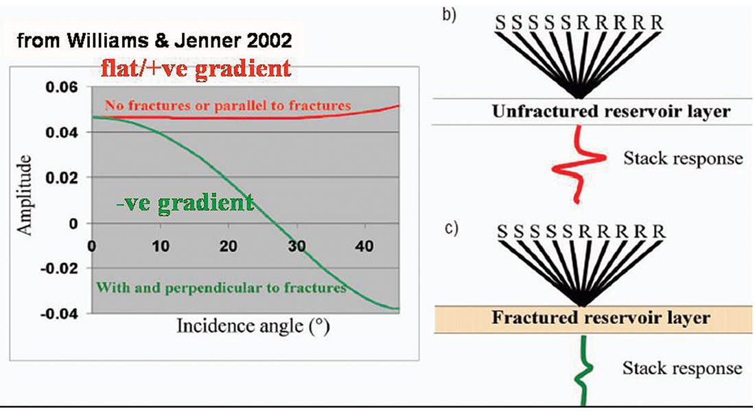
All these examples suggest that anisotropic effects are commonly observed in seismic data. However there is no unambiguous relationship of AVAZ gradient to either the orientation of fracture azimuth or the intensity of the anisotropy. This can be seen by comparing figures 1 and 3 with an increasing (positive) or flat gradient perpendicular to fractures and a decreasing (negative) gradient parallel to fractures to the opposite case in figure 2.
Figures 4 and 5, that are both examples of fractured carbonates, show a similar conflict with the fracture perpendicular orientation having a relative increase in gradient strength for the Weyburn reservoir, while the stronger gradient is in the parallel alignment in the other example from Todorovic-Marinic et al.
The problem is that without any additional geological or log information indicating the presence of fractures, interpretation of the seismic AVAZ observations alone could be misleading or wrong for both orientation and intensity.
Despite these ambiguities in the data the AVAZ interpretation for fracture orientation and intensity prediction can be established by modeling and theory as shown in figures 6 and 7a. But even here there is a conflict with no single and obvious guiding principle. The Williams and Jenner model in figure 6, is compelling as it logically explains the expected weaker 3D stack response to fractures. This is shown to be the result of a decreasing (negative) gradient perpendicular to strike, while the isotropic or parallel case has a flat gradient and hence a strong stack response for CDP’s in areas where no fractures exist. This conclusion is exactly opposite to a rule of thumb suggesting that the direction of the lesser AVAZ gradient is parallel to fracture strike (Thomsen 1995). It is interesting to note that this lack of generality is unlike the isotropic AVO type gradient classification that is diagnostic of changes in Vp/Vs ratio and may be the reason why conventional AVO is the more widely used technology.
The reality is that there is no rule of thumb and in order to better understand these ambiguities one needs to delve into the theory that has been primarily developed by Ruger and Tsvankin (Ruger 1997). Figure 7a shows the AVO gradient variation with azimuth for two models with different anisotropic parameters from Ruger’s Leading Edge paper that are based on the linearized azimuthal AVO equation that he developed.


A few initial observations are that:
- the magnitude of the gradient variation with azimuth is much smaller than the overall basic isotropic AVO gradient despite a realistic choice of values for anisotropic parameters between 8% and 15%,
- the magnitude of gradient variation with azimuth shown in both the data and model examples in figures 1 to 6, are significantly larger than those predicted by Ruger’s equation even to the point of reversing the sign of the gradient (compare figures 7a and 7b),
- the relative stack response from a fractured vs. isotropic layer can be consistent or at odds with one’s intuition (compare figure 6 to figure 7b),
- the zero offset reflection has no azimuth variation.
The following sections cover the theory behind Ruger’s azimuthal AVO equation and the impact of the anisotropic parameter values that lead to the ambiguities in data and models shown and described above.
Anisotropic AVO Theory and Models from Ruger’s equation
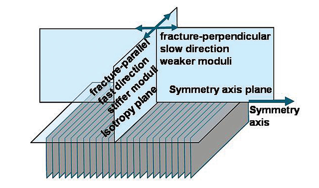
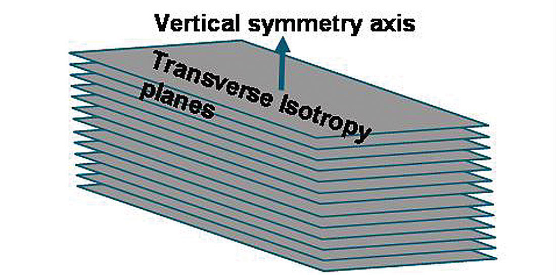
Inversion for anisotropy using P-wave data follows from conventional isotropic AVO by utilizing Ruger’s anisotropic reformulation of the Aki and Richards linearized equation for P-wave reflectivity with incidence angle (Aki and Richards 1980, Ruger 1997). This reformulation is based on a simple model of vertically aligned fractures termed HTI (horizontal transverse isotropy) as shown in figure 8. The HTI model is identical in its transverse isotropy (TI) to the more familiar vertical transverse isotropy (VTI) model for horizontal layers e.g. shales, with the only difference being a 90° rotation of the symmetry axis from vertical to horizontal (see figures 13 a and b, in the following section).
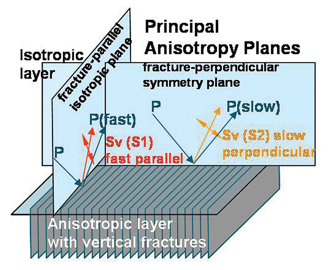
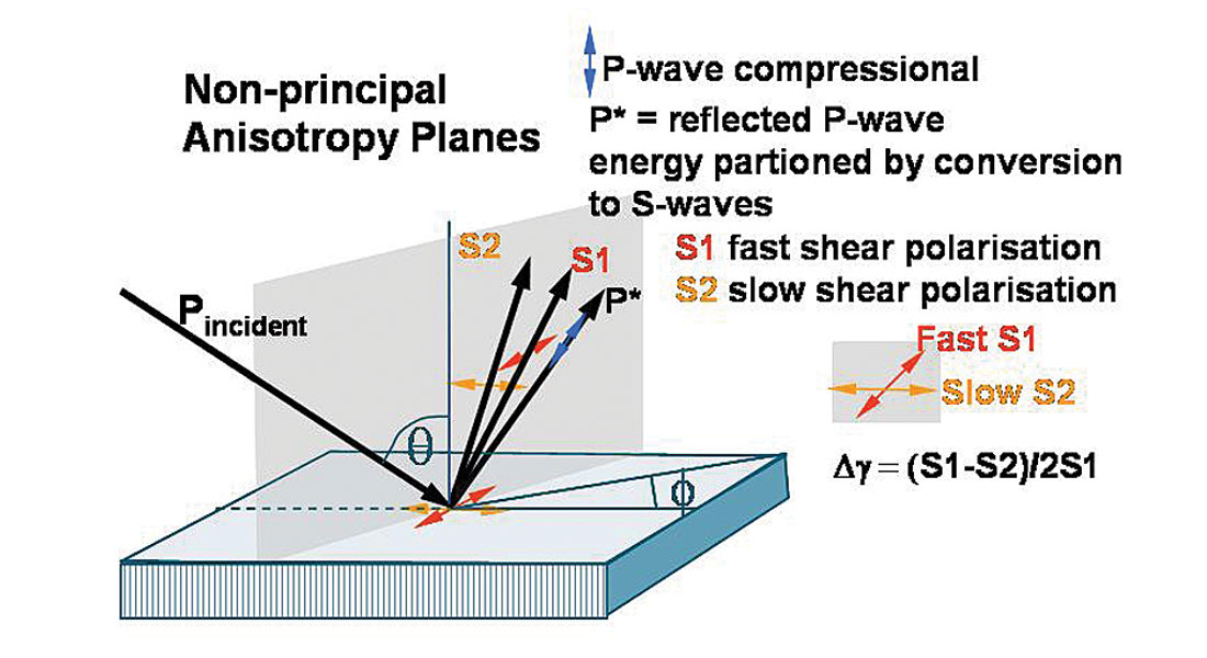
Just as conventional isotropic AVO is a consequence of P-wave energy conversion to vertically polarized Sv shear-waves at a reflecting boundary, so the azimuthally anisotropic equivalent converts to a fast Sv (S1) shear-wave in the principal isotropic plane and a slow Sv (S2) shear-wave in the anisotropic symmetry axis plane, as shown in figure 8. At azimuth angles between the principal planes, conversion occurs to both a fast S1 and a slow S2 shear-wave, polarized parallel and perpendicular to the fracture strike or maximum stress direction respectively. This polarization that gives rise to the S1, S2 velocity difference, is termed shear-wave splitting and is defined as a percentage measure of shearwave anisotropy by Thomsen’s γ parameter (Thomsen 1986).
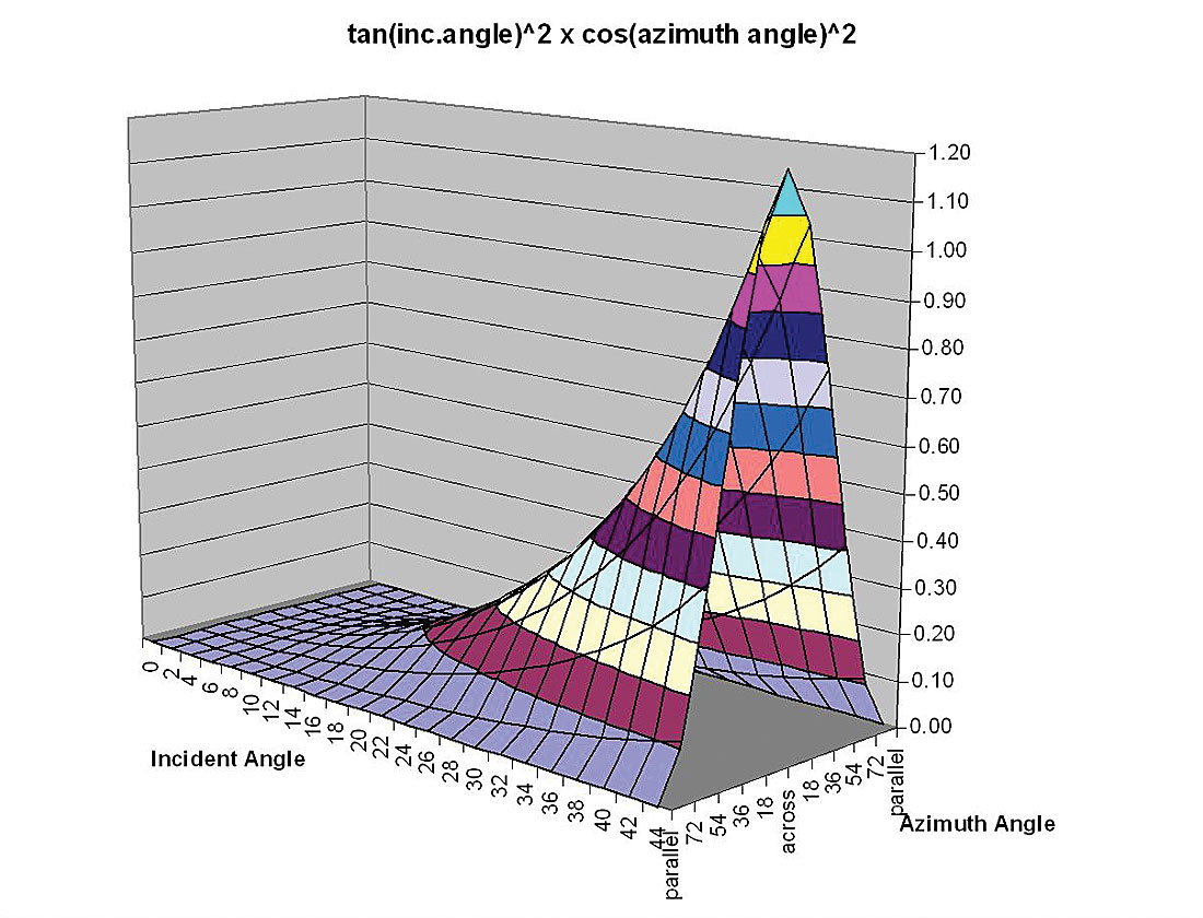
At large propagation angles relative to vertical both P-waves and shear-waves are impeded in the anisotropic HTI symmetry axis plane i.e. the minimum stress direction or perpendicular to fracture induced layering. This results in a progressive reduction in impedance contrast with azimuth from the isotropic to the symmetry axis planes, for high incidence angle reflections. However in the vertical axis of the HTI media P-waves propagate at the fastest velocity in the fractured layer with no shear-wave conversion at the reflection boundary, whose coefficient is equal to that of the normal incidence P-reflection from the highest isotropic impedance contrast. In the symmetry axis plane at increasing incidence angles, P-wave propagation velocity decreases to a minimum for horizontal propagation along the HTI symmetry axis. This can be seen to be equivalent to the familiar VTI model (with the 90° symmetry axis rotation) where the difference between vertical and horizontal P-wave propagation phase velocity is described by Thomsen’s ε (epsilon) parameter. In a similar analogy between the symmetry axis planes for VTI and HTI, P-wave propagation phase velocity is further described by Thomsen’s δ (delta) parameter for non-normal incident angles with a maximum effect at 45°. The influence of ε and δ on P-wave phase velocity and gamma γ on shear-wave phase velocity (i.e. the velocities involved in impedance contrasts and hence AVO reflection coefficients), are shown in equation 1 below for the VTI case.
where θ = incident phase angle α0 β0 = vertical P-wave and shear-wave phase velocities respectively.
However for the HTI model both ε and δ undergo a transformation to ε(v) and δ(v), where (v) denotes a vertical axis reference due to the 90° symmetry axis rotation from their VTI equivalents as given in equation 2 (Ruger 1997, for explanation and derivation see the following section).
Consequently these HTI parameters ε(v) and δ(v) along with the VTI γ, appear in Ruger’s HTI AVAZ reflection equation (amplitude vs. incidence and azimuth angle) for azimuth angles ϕ between the principal symmetry axis and isotropy planes as shown in equation 3.

where:

Incidence angle θ, α0 and β0. are averaged across reflection interface between HTI and overlying layer.
HTI Thomsen parameters Δγ, Δε(v) and Δδ(v) are differences in anisotropy from HTI to overlying layer.
ϕ= azimuth angle with respect to symmetry axis plane where ϕ=0.
For the isotropic plane, equation 3 follows the reformulation of the three term Aki and Richards AVO equation shown in part 1 as equation d (Wang 1999, Goodway 2000) this being based on vertical fractional contrasts or reflectivity in density Δρ/ρ, P-wave velocity Δα/α and rigidity Δµ/µ.
However Ruger chose to follow the approach of Shuey (equation c, in part 1) by gathering the Δα/α, Δε(v) and Δδ(v) terms with significant contrast (Ciso Caniso in equation 3), into the third higher order incidence angle sin2θ tan2θ term. The consequence of this is similar to the isotropic case shown in part 1 in that both AVO and AVAZ equations do not have the critical curvature discrimination when used in industry practice as two term approximations (see figure 11a). However as will be shown later, the relative contribution of the 2nd vs. 3rd term is far worse of a problem in the AVAZ case leading to fundamental ambiguities and hence errors involved in azimuthal anisotropy inversion based on Ruger’s equation. This also explains the wide variation and basic confusion in observation or interpretation of AVAZ effects in the data and model examples shown in the previous section.
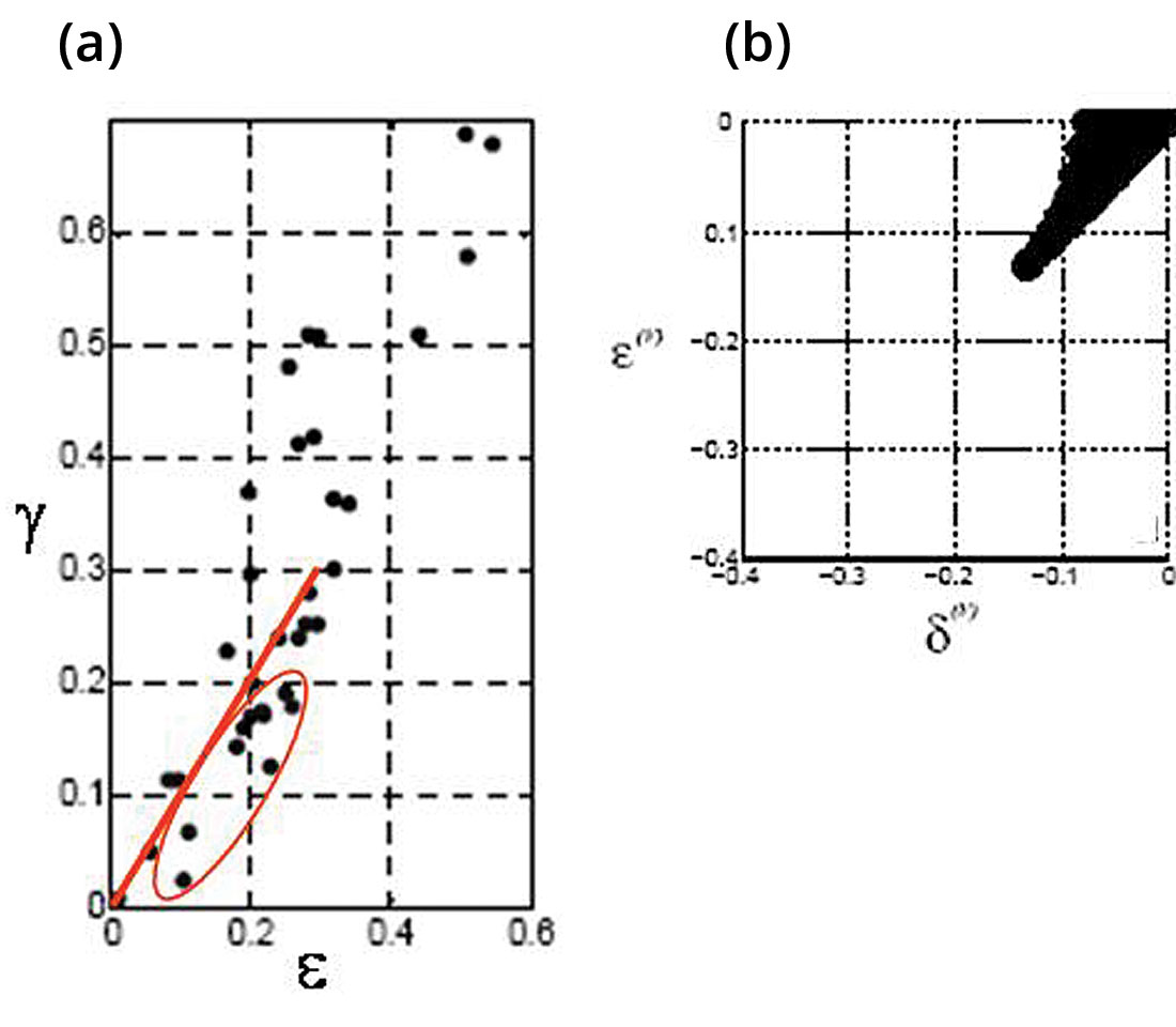
Figure 9b). Relationship between values of HTI fracture model parameters ε(v) and δ(v), for ranges of |γ(v)|< 0.05 (from Bakulin et al., 2000).
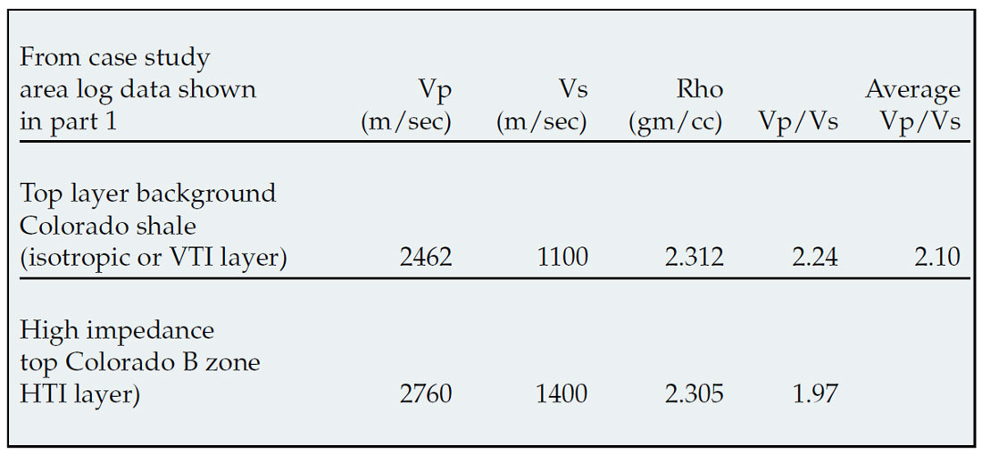
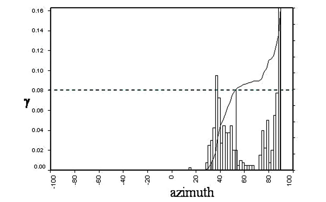
In order to demonstrate this problem, P-wave, shear-wave velocities and density based on the log data shown for the Colorado case study in part 1, are used to model an isotropic/HTI layer boundary (see table 1). Maximum values of γ=0.08 for shear-wave splitting were established from dipole log measurements shown in figure 10 for the Colorado gas shale. Other realistic values for HTI anisotropy are chosen for the case of shales with low porosity where relative values of γ/ε= 0.8 can be established from figure 9a, circled below the red line for γ < 0.2. A gas filled fracture model is further characterized by elliptical anisotropy where ε(v) = δ(v) (Ruger 1997, Bakulin et al., 2000) which along with the relationship shown in figure 9b, leads to ε(v) = δ(v) = -0.1.
Using the values established above, figures 11a and b, show the AVAZ curve variation with incidence angle from parallel (isotropic plane) to perpendicular (symmetry axis plane) for an isotropic/ HTI model, comparing the 2 term (A and [Biso+Baniso]sin2θ) Shuey type approximation as used in practice, to the full 3 term Ruger equation 3.
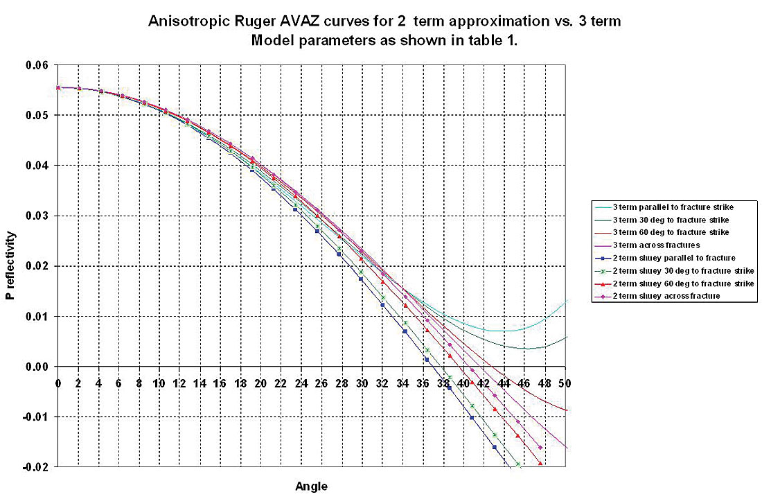
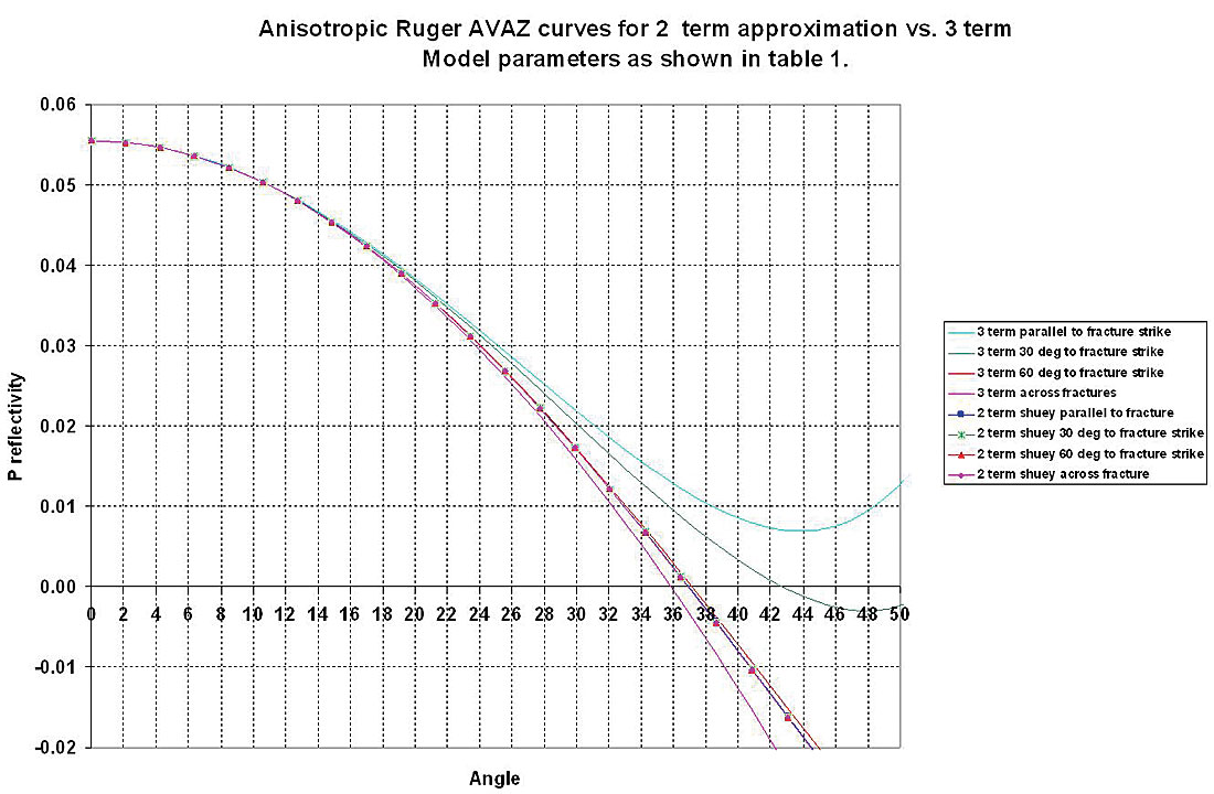
The following observations can be drawn:
- The full 3 term curves are similar to those shown by Ruger for gas filled fractures with similar HTI parameters (γ = 0.085, ε(v) =-0.15 and δ(v) = -0.155, see right panel of figure 7a above) where very little separation can be seen between the curves for varying azimuth for incidence angles up to 35°. However at reasonably large angle ranges between 35° to 45°, discrimination between azimuths is possible due to the curvature in the 3 term equation. The curvature diminishes with decreasing azimuth angle ϕ from parallel to fractures ( isotropic plane) to perpendicular or across fracture s (symmetry axis plane).
- The two term approximation used in practice shows a large and opposed separation in azimuth AVO curves for most of the incidence angle range from 20° to 45° and is unable to match the critically diagnostic 3 term curvature beyond 35°.
- The most startling observations are that using a 2 term Shuey approximation to fit the actual 3 term measurement would produce a result that showed no azimuthal anisotropy for angles less than 35° and the wrong opposed 90° fracture azimuth for angles greater than 35° !
These conclusions seriously undermine the ability of the AVAZ method as used in practice, to correctly detect the orientation and degree of anisotropy from a fracture or stress induced HTI model.
However a better understanding of the limitations of these ambiguities can be obtained through the following analysis of Ruger’s equation thereby leading to improvements in the ability of the technology to establish the degree and orientation of anisotropy that is critical to the drilling these tight gas Resource Plays.
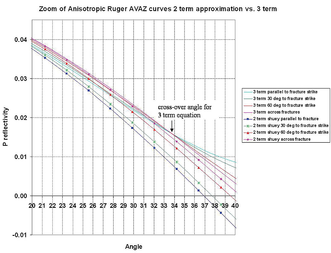
The reason for the results and observations shown above for the gas filled fracture model, is that the 2nd term in Ruger’s equation (equation 3) is reduced in significance below θ = 35° incidence angle, as a result of the Baniso term having anisotropic parameters γ and δ(v) with opposite sign (see equation 2). Consequently the 3rd high incidence angle term (CisoCaniso in equation 3) has more impact on the azimuthal gradient and cannot be ignored. In fact in a yet more ambiguous way a “cross-over” angle occurs at 33.9° where for θ < 33.9° the “parallel to fractures” (isotropic) azimuth AVO curve is below that of the “perpendicular to fractures” (symmetry axis plane) curve and reverses this sense for θ > 33.9° with a greater, more visible separation (see figures 11b: 3 term panel and 11c: zoom-in of figure 11a).
Ruger’s equation can be rewritten to separate the isotropic terms from anisotropic terms in order to explain the AVAZ curves in figure 11 a, b and c as follows.
For the gas filled fracture case being considered here for elliptical anisotropy, the anisotropic term becomes:
Where as mentioned above there exists a “cross-over” incident angle (θ) of zero azimuthal (ϕ) amplitude variation (see figure 11a and b) whose value can be found from:
where for values used in the Colorado gas shale model of gas filled factures of:

Despite the sense of the azimuthal AVO gradient being complicated by a dependence on an incidence angle cross-over point, there is also the potential to use this knowledge to look for a cross-over angle in offset-azimuth (angle) cube displays such as figure 11b. If such a cross-over angle exists, i.e. where all azimuths have the same reflectivity, then the HTI anisotropy is likely to be near elliptical ε(v) ≈ δ(v) and the γ / ε(v) ratio can be estimated from tan2θ as shown, knowing the average Vp/Vs ratio.
In fact just such a cross-over incidence angle is visible at a little less than 1800m offset in the offset-azimuth cube display of the Weyburn fractured Midale carbonate reservoir shown in figure 4 (strong band of red across all azimuths marked as cross- over angle points).
An appreciation of the sensitivity of Ruger’s equation to changes in ε(v) and δ(v) can be seen by comparing figures 11a to 11d, where a change from ε(v) = δ(v) =-0.1 to -0.145 has the effect of removing all azimuthal gradient variation in the 2 term approximation while significantly increasing the 3 term variation.
Given the importance of the 3rd term in Ruger’s equation from the foregoing discussion, a better approach would be to rewrite the equation in three terms of equal significance. The result shown below in equations 5 to 6, follow from the equivalent isotropic equation c, in part 1 (Wang 1999, Goodway 2001) with a zero incidence angle term in Δα/α and two isotropic / anisotropic terms in sin2θ (including Δµ/µ) and tan2θ (including Δα/α). For the elliptical case (equation 6) the underlying physical connection of the impact of the HTI anisotropic parameters Δε(v) (-ve sign) and Δγ (+ve sign) can be seen as respectively reducing the isotropic AVO gradient terms for Δα/α and Δµ/µ, as these are the parameters associated with the P-wave VTI phase velocity and shear-wave splitting shown in equation 1. Note that the factor of 2 for the Δγ term is a function of its combination with rigidity that is related to the shear-wave velocity squared, unlike Δε(v) with Δα/α.

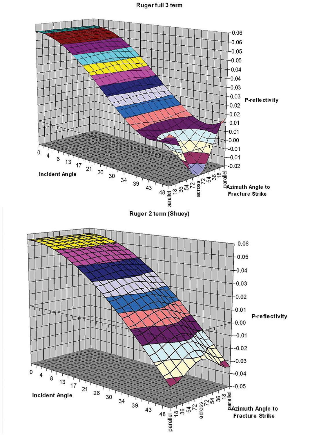
A relatively robust 3 term method for inversion of azimuthal anisotropic parameters based on equation 5 would progress in the following sequence below, as there is enough separation between the 2nd term’s tan2θcos2ϕ surface and the 3rd term’s sin2θcos2ϕ surface shown in figures 12a and b.
- estimate the zero angle reflectivity to obtain Δα/α
- estimate an initial symmetry-axis plane direction from the azimuth gradients at relatively high incidence angle θ = 40°(see figures 12 a, and b)
- 3) estimate Δµ/µ from the isotropic azimuths in a standard AVO “weighted-stacking” approach (Gidlow et al., 1992)
- extract an estimate of Δε(v) by comparing the δ α/α scaled tan2θ curves between the isotropic plane and the symmetry-axis plane or by fitting a Δα/α scaled tan2θcos2ϕ surface (figure 12 a)
- obtain the sin2θcos2ϕ surface (figure 12 b) by subtraction of the tan2θcos2ϕ surface (figure 12a) from the full azimuthal AVO gradient surface estimate
- extract an estimate of Δγ from the difference between the Δµ/µ scaled sin2θ curves for the isotropic plane and the symmetry-axis plane or by fitting a Δµ/ µ scaled sin2θcos2ϕ surface (figure 12b)

alternatively with the following substitution based on equation 2
Next by dropping the small constant Δρ/ρ term (see equation c, in part 1) and for elliptical anisotropy (the gas filled fracture case under consideration) Δδ(v) = Δε(v)
and for elliptical anisotropy where Δε(v) ≈ 0
VTI-HTI anisotropy, moduli and Thomsen parameters.
In order to gain further insight into the ambiguities of Rugers P-wave azimuthal AVO equation shown in the previous section, it is necessary to understand all three Thomsen (1986) parameters ε, δ and γ, involved in the anisotropic variation of AVO gradient for VTI media and their HTI equivalents.
The model of anisotropy describing a single set of vertical fractures, is that of Transverse Isotropy (TI) with a horizontal axis of symmetry termed HTI (see fig. 13a). This model has five independent constants or moduli denoted by stiffnesses cijkl, that quantify the stress to strain ratio and are rank 4 tensors i.e. relating the rank 2 stress σij to strain ekl tensors in Hooke’s Law given as:
with indices j and l being normals and i and k the directions of stress or strain in a Cartesian system of z, y and z shown in the diagram

The cijkl’s contain the Lamé parameters or moduli of incompressibility Lambda (λ) and two rigidity Mu (µ) terms. These moduli are combined for specific directions of stress to strain tensors, constrained by the Kronecker delta functions (note these δ’s are not Thomsen’s delta and from here on δ represents Thomsen’s δ). Cijkl's or moduli can also be described in a stress-strain tensor matrix, where the simplest isotropic case involves only two moduli (λ and µ) as shown below.
Following from the expression for Hooke’s law this matrix can be expressed in Lamé terms as:
Thomsen initially developed his parameters for TI media as an equivalent homogeneous continuum representing fine layering e.g. shales, with a vertical symmetry axis (VTI as shown in fig.13b). Following this model the five term anisotropic VTI stress- strain tensor matrix is considered first by analogy with the isotropic case:
This matrix can be represented in Lamé terms in two ways modified from Sheriff’s Dictionary of Geophysics (1991 page 99).
Case (1) as given by Sheriff:
Where ≡ is measured parallel to layering, ⊥ is perpendicular to layering and * denotes a third independent rigidity modulus µ*.
Using the cijkl to Lamé moduli relations shown in the last pair of VTI matrices above, Thomsen’s δ as defined in his 1986 paper, can be represented as:
From this δ is seen to be a function of the difference between µ* and µ⊥ in the numerator and if µ* = µ⊥ then δ = 0.
Next Thomsen’s gamma γ, that controls shear wave splitting and therefore also appears in Rugers’ equation, is similarly represented as:
However a more generally accepted interpretation of shear wave splitting in terms of γ is to consider the numerator in the above equation as the difference in layer parallel µ≡ to layer perpendicular µ denoted as µ⊥ not µ*. Further support for only two µ terms is given by Schoenberg (Schoenberg et al., 1996) where VTI symmetry is approximated to three terms described by an isotropic λ and only two µ terms i.e. µ≡ and µ⊥.
Also in the context of the shear wave splitting parameter γ used by Ruger in his AVAZ equation, the assumption is that only two µ’s (µ≡ and µ⊥) describe the shear wave anisotropy as shown in Thomsen’s 1986 formulation for shear wave phase velocities or vsh waves (polarized in the horizontal plane having Voigt index xy):

So assuming the generally accepted case where µ* = µ⊥ with only µ≡ and µ⊥ describing the anisotropic rigidity, a second possibility for Sheriff’s tensor matrix can be formulated as follows.
Case (2):

Here as before ≡ is measured parallel to layering and ⊥ is perpendicular to layering, while Lambda λ13 and Lambda λ33 are contained in stiffnesses C13 and C33.
So with this version of Sheriff’s matrix and again by comparison to the above VTI matrix in cijkl terms, Thomsen’s delta δ can now be represented in Lamé terms as:
This relationship now reveals δ as being a function of the λ13-λ33 difference. The significance of this difference in anisotropic Lambda’s can be understood by considering a VTI version of Hooke’s law for axial stress in the vertical z-direction given as:

From this equation the difference in λ13 and λ33 can be seen as representing the difference in axial strain ezz to either transverse strain exx or eyy, from Lambda terms alone, unlike the isotropic case where the contribution of stress to axial and transverse strains is equal. This suggests that δ is influenced more by variations in Lambda due predominantly to the incompressibility of the fluid fill between the solid layers in the VTI or HTI models shown in figures 13a, and 13b (Berryman et al., 1999).
It is interesting to note that in Thomsen’s DISC 2002 manual he states on page 1-21 “… λ does not have a common name, since it is not useful for much in geophysics (despite what you might have heard!).” In the context given here one might also add that if λ is not useful for much in geophysics then neither is δ as it is strongly influenced by λ.
Finally to complete the VTI parameterization, Thomsen’s epsilon ε, the P-wave equivalent to γ, is given as:
The last expression shows a relationship between ε and γ where generally ε > γ as the difference λ = – λ⊥is positive and generally large. This understanding forms the basis for the choice of anisotropic values used to create realistic gas charged HTI model values for Ruger’s azimuthal P-wave AVO gradients shown in the previous section (see figure 9a).
To this point, only the VTI matrix has been considered and the descriptions for Thomsen’s epsilon ε and δ are derived for the VTI matrix based on a vertical axis of symmetry (fig 13b). In the HTI model (figure 13a) used for Ruger’s equation, ε and δ are replaced by ε(v) and δ(v) being a function of the horizontal symmetry axis as opposed to the vertical VTI case. The symmetry axis rotation gives rise to values for ε(v) and δ(v) that are now of opposite sign to γ and the original ε and δ, leading eventually to ambiguities in Ruger’s azimuthal AVO gradient equation as shown in the previous section. This change in sign can be understood by considering a transformation of the VTI matrices in cijkl and Lamé moduli terms, from a vertical to horizontal symmetry axis.
The resulting equivalent HTI matrices to the VTI matrices given above are:
and represented similarly in Lamé terms as:
Where as before ≡ is measured parallel to layering and, ⊥ is perpendicular to layering that is now in the vertical plane.
Following Ruger 1997, the ε to ε(v) relationship can be derived using the cijkl to Lamé moduli relations shown in this last pair of HTI matrices as follows:
Starting from the HTI matrices above
and from the VTI (case 2) matrix where λ33 ⇒ λ⊥
The resulting expression for ε(v) shows that because of a rotation of the symmetry axis by 90° in going from VTI to HTI, so consequently ε(v) has a negative sign compared to ε that is positive for VTI.
Finally it can be shown through a similar derivation that the δ to δ(v) relationship is:
Starting from the HTI matrices above
The final expression relating δ(v) to δ given as δ(v) = {(δ -2ε)/(1+2ε)}{(f+ε)/(f+2ε)} also shows that because of a rotation of the symmetry axis by 90° in going from VTI to HTI, so δ(v) has a negative sign compared to δ and ε, as ε is generally greater than or equal to δ and both are positive for VTI.
It is these changes in sign for ε(v) and δ(v) due to a transformation from VTI to HTI that create the ambiguity in Rugers AVAZ equation as described in the previous section.
Case study of 3D AVO and AVAZ inversion, coherency mapping and subsequent drilling results
This final section describes the results of 3D AVAZ and coherence mapping from the study area described in part 1, tied to the subsequent drilling and a full dipole/FMI log suite.
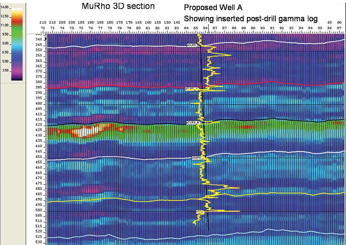
Despite the somewhat un-encouraging analysis in the previous sections of industry’s AVAZ practice in using a “Shuey type” 2 term version of Ruger’s azimuthal AVO gradient, an AVAZ inversion to estimate fracture density and orientation was run on the 3D in the study area. The proposed deviated well location (Well A) was initially chosen by identifying the most fracture prone high MuRho zones (see part 1 and figure 14 here).
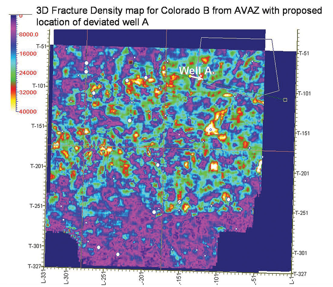
This was then combined with faulting implied from 3D coherence attribute lineations (figures 16 a and b) along with the addition of the AVAZ fracture density map (figure 15), as these independent attributes provided powerful corroborative evidence of fractures at the proposed location.
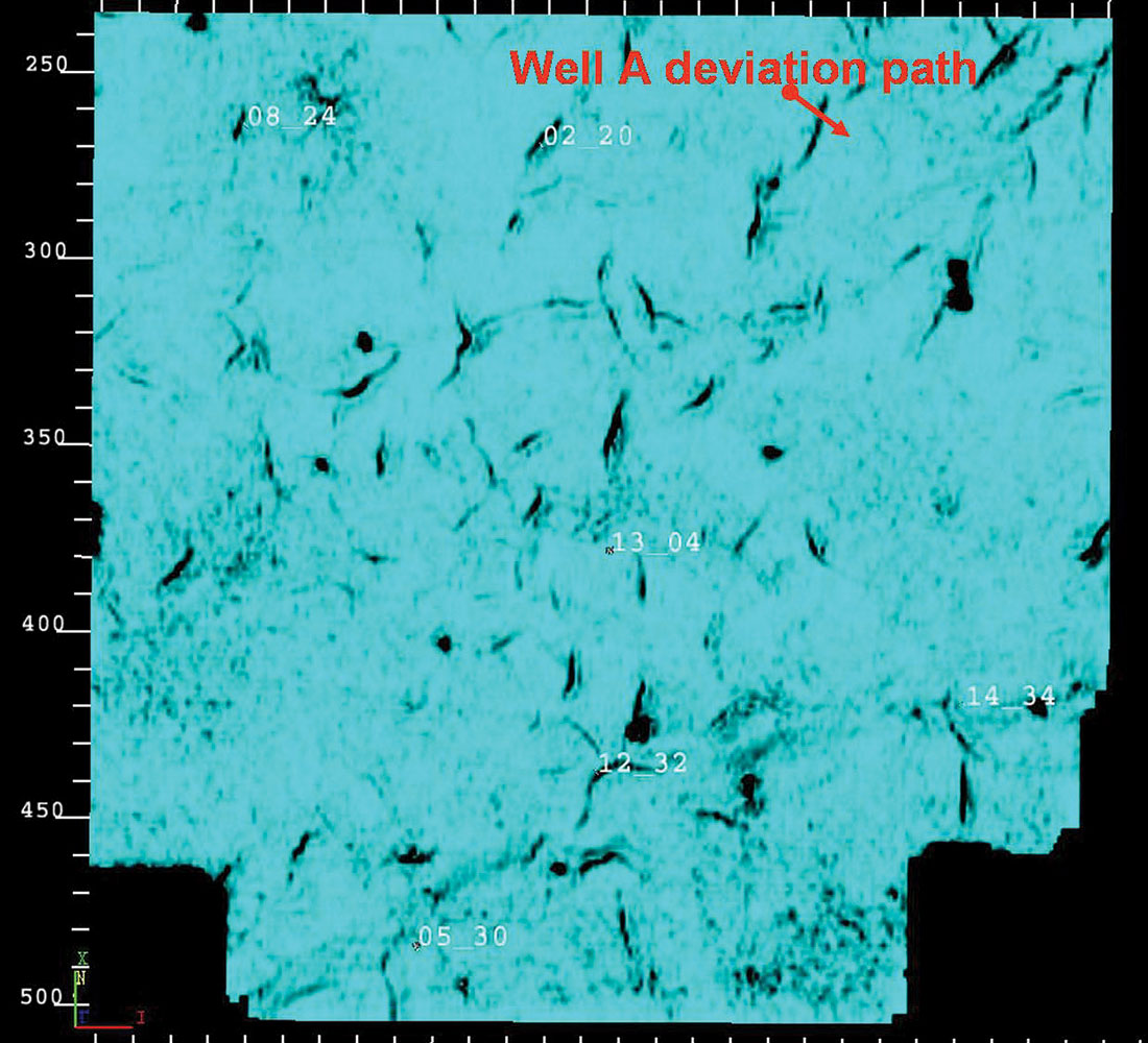
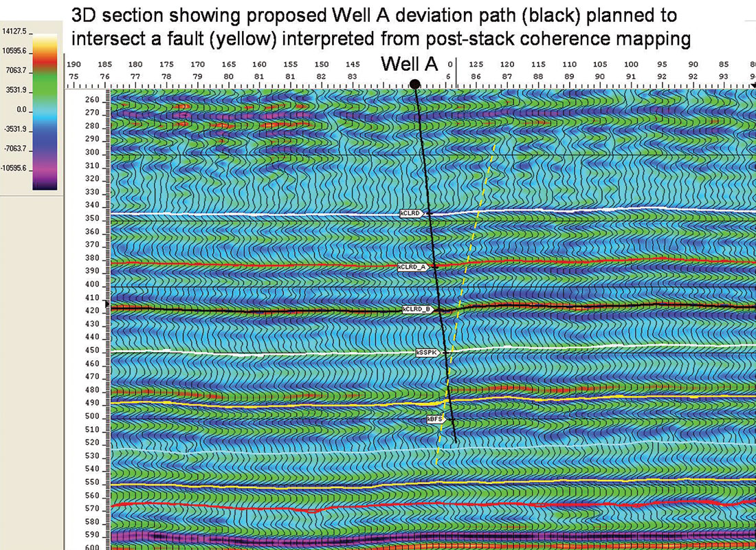
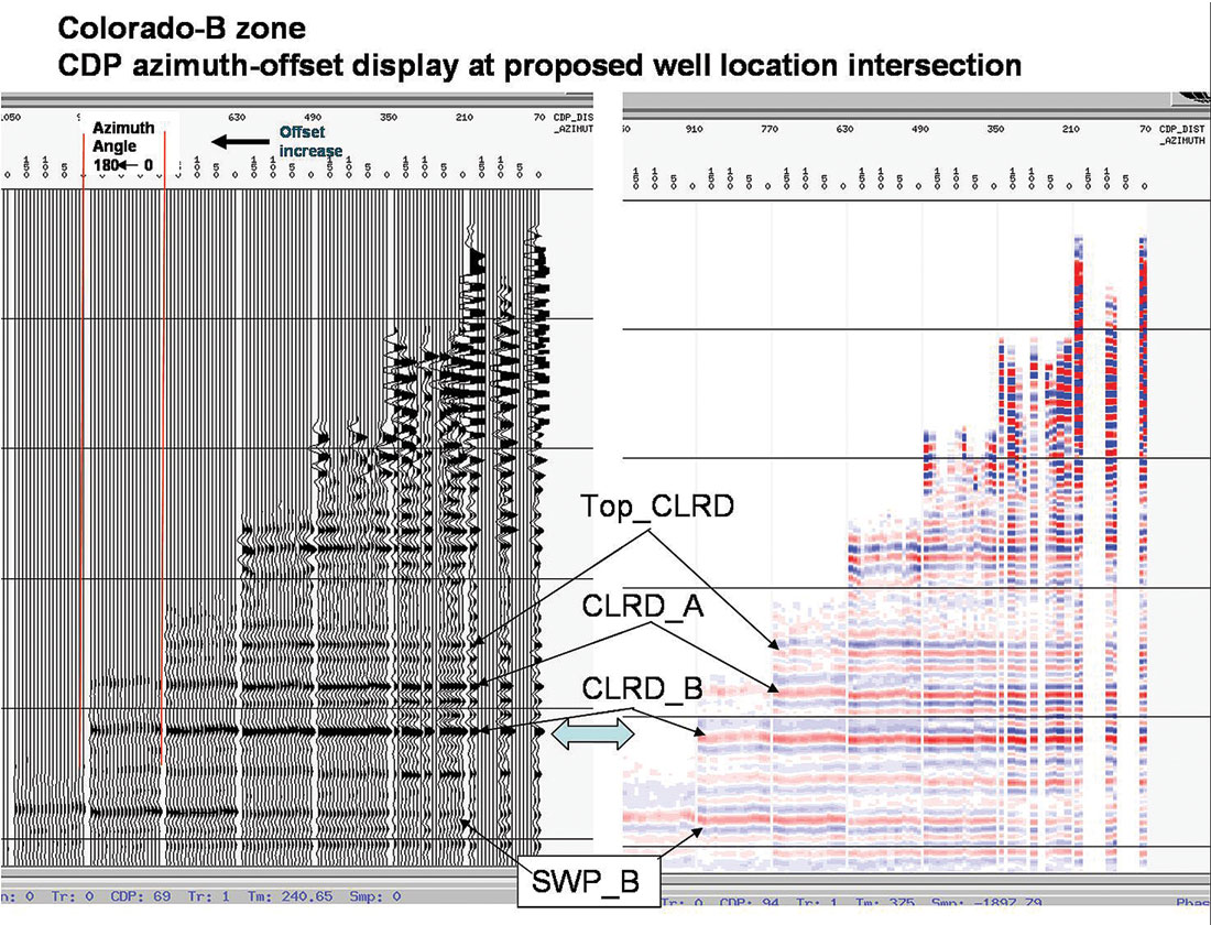
Figure 17 shows an azimuth-offset display of a CDP at the proposed Well A location where distinct and theoretically correct AVAZ amplitude variation can be seen at the Colorado B level.
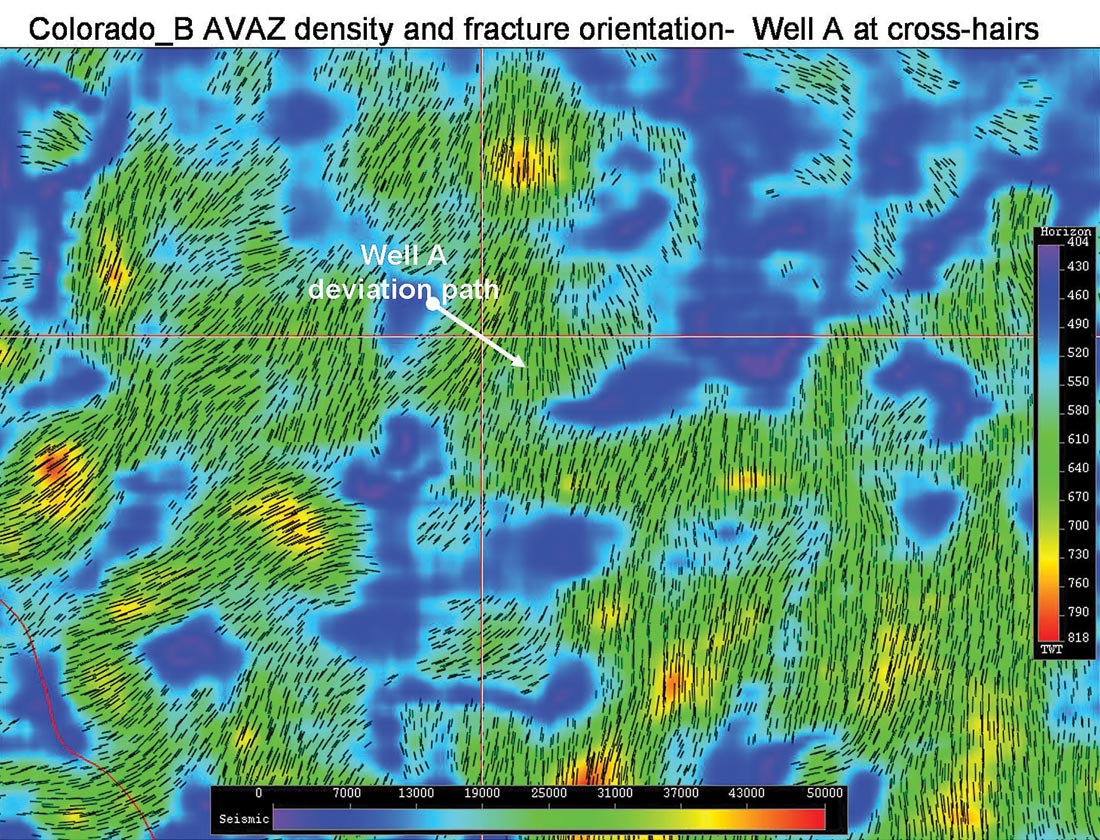
A detailed 3D map of fracture density (colour intensity) and orientation (“iron filings” tick marks) in figure 18, shows an excellent match with the direction of the coherence attribute lineament shown in figure 16 a.
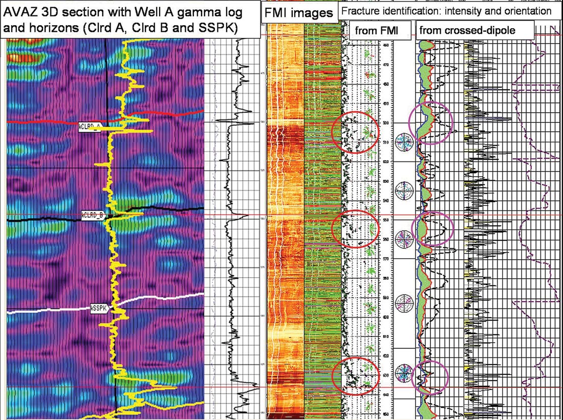
In conclusion for this case study, the outcome of drilling Well A perpendicular to fracture prediction from AVAZ and coherence, was positive with the deviated well-bore encountering fractures at the Colorado B level as predicted. The seismic vs. log results are shown in figure 19 where the left AVAZ attribute panel clearly shows high fracture density (hot colours) at the Colorado A, B and below the 2nd White Specks (SSPK) levels that are confirmed by the red circles on the middle tracks for FMI interpretation and pink circles for crossed-dipole anisotropy measurements shown in the rightmost tracks.
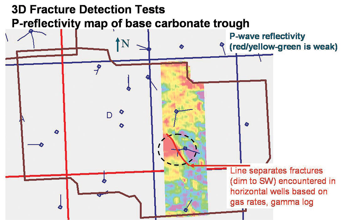
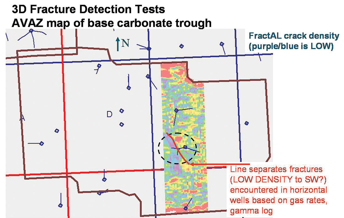
However this paper would not be complete given all the fundamental ambiguity involved in Ruger’s 3 term AVAZ equation and industry’s 2 term approximations, without a final example that shows a miss-match between areas predicted as fractured from azimuthal AVO attributes and fractures established from horizontal drilling of basic P-wave stacked amplitudes. Figures 20 a and 20 b (courtesy of Doug Anderson an interpreter at EnCana) show how the AVAZ fracture density map predicts exactly the opposite areas for fractures when compared to the P-wave stacked amplitude. In this case the P-wave amplitude was correct as confirmed by horizontal drilling also shown in the comparison. The problem shown in figures 20 a and b, of miss-matching AVAZ maps based on a 2 term azimuthal AVO gradient fit, with the more intuitive P-wave stack response to fractures, is a good example of the ambiguities described in the theory section at the beginning of this paper and is similar to the confusion shown in the section on “Examples of Azimuthal AVO” from the literature.

Acknowledgements
Dave Gray, Dragana Todorovic-Marinic and Jay Gunderson (Veritas DGC).


Join the Conversation
Interested in starting, or contributing to a conversation about an article or issue of the RECORDER? Join our CSEG LinkedIn Group.
Share This Article