Playing with Fire: Trim Statics and Noise Alignment

Summary

The danger of noise alignment in trim statics is reviewed and illustrated. Such noise alignment is then quantified through numerical studies to obtain a clearer understanding of this phenomenon. The results are used to quantify an allowable range of trim statics for a given acquisition geometry, and to develop tests for detecting potential noise alignment in aggressive trim calculations.

Introduction — The Danger of Noise Alignment

The summing of traces in a common midpoint (CMP) gather assumes the reflection data is aligned and the amplitude will increase with the fold or number of traces in the gather. Noise will also sum, but its amplitude will increase with the square-root of the fold. The corresponding gain in the signal to noise ratio (SNR) will be proportional to the square root of the fold. Thus it may be assumed that a high fold will give better results. However when the reflection data is misaligned, poor results with a lower SNR may be obtained instead. The objective of estimating statics is to align the reflection data to improve the SNR of the stacked section.

To accomplish this, each trace in a gather is cross-correlated with a pilot trace, which we assume has been constructed to represent what the gather traces ‘should’ look like (a simple stack of traces is often used). The maximum of the cross-correlation function gives us the information necessary to align the traces to be more coherent with each other. The underlying assumption is that one is aligning the signal in the various traces. Unfortunately, the same processes may result in aligning the noise component to match the pilot trace as well, resulting in an apparent SNR which is higher than the true SNR.

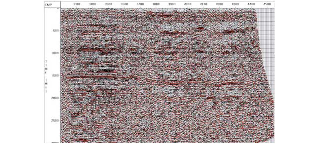
To illustrate, a stacked section (from Asia) is examined with a best processing stack shown in Figure 1. The average maximum fold in each trace is above 100. The structure in the data will be assumed to be due to a surface static and trim statics will be applied to remove the apparent structure. A very large correlation window of 2.0s will be used to eliminate problems typically associated with trim statics. A large maximum time shift of ±250 ms will be used to allow the reflection data to be aligned. (Both are bad assumptions). A model trace is found by stacking 25 traces from the stacked section in Figure 1 (in the area of CMP3400) that appear to have stable reflection energy.

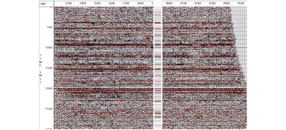
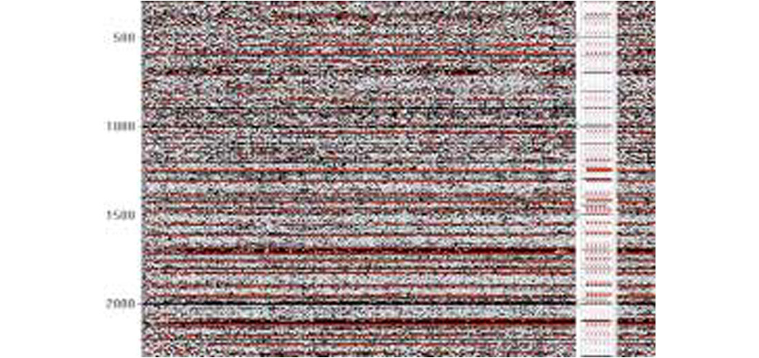
The resulting trimmed section is shown in Figure 2. Note the horizontally aligned data and how well it corresponds to the model trace that is inserted in the middle of the section. Obviously the assumption of surface statics is correct (only in the mind of the data manager) and the trim statics has produced a very good section, even in areas where the original section is poor. The only problem is that there is no structure in the data for prospective drilling.

The crafty processor, however, chooses new data from Alberta to form a new model trace. Using the same parameters as above, another stacked section was created (displayed in Figure 3) with equally as good an appearance as Figure 2. The continental drift theory may be correct and Alberta was once connected to …

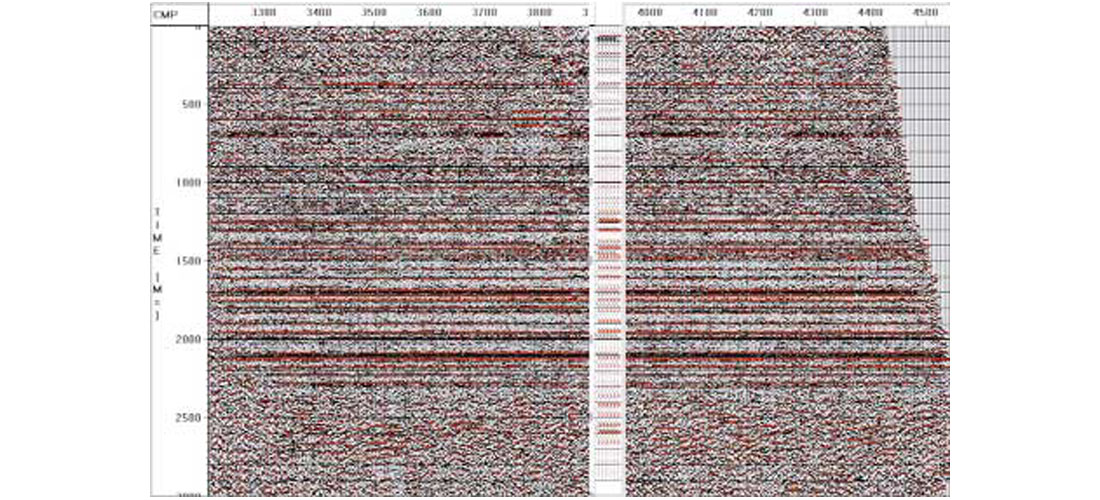
Clearly the trim static, when applied directly to this data, has only aligned the noise to produce a section that matches whatever model trace it is given, and then only within the correlation window. Hence the usual practice of choosing very small maximum shifts. Unfortunately, there are sometimes cases when large maximum shifts may be desirable. In some data, such as the Sahara, there can be large surface statics, and it may be unclear whether the apparent structure is real, or simply the result of very large residual statics.

Generally when large residual statics are estimated they are decomposed into source and receiver components to avoid noise alignment, and only trim statics that are less than, say, 6 ms are directly applied to the data. In this paper we explore whether an increased understanding of noise alignment will allow us to use larger trim statics alone, without any surface consistency requirements (and without getting burned in the process!).

Quantifying Noise Alignment

To better understand the degree to which noise is aligned we will first generate a data set consisting entirely of random noise. Using this data we will carry out trim statics with various sets of parameters. This will give results that can be generalized into an expression [Eq. (4)] which quantifies the expected alignment of noise in any trim statics operation.

A recipe for pure noise data

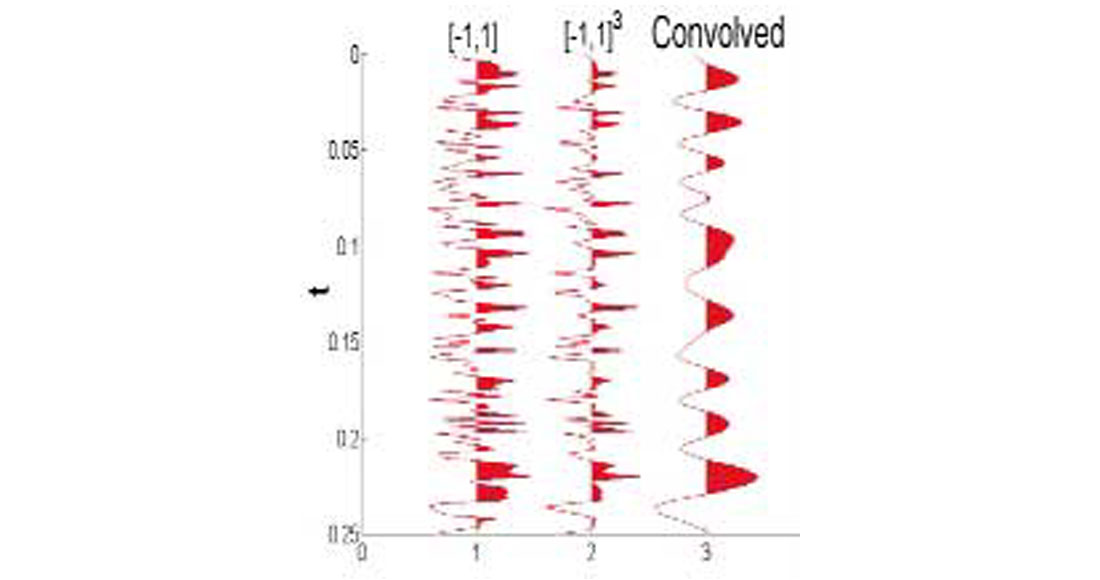
A sample random noise data trace is displayed in Figure 4, where we also illustrate the procedure used to create it (see figure caption). This procedure is carried out 10n times to create 10 synthetic CMP gathers, each with n traces. This data is then trimmed for various values of n.

Trimming the noise and estimating its apparent SNR ratio

To apply trim statics we first generate a pilot, or reference, trace. Normally this is generated from the CMP gather, but in this case it will be a random data trace, generated by the procedure illustrated in Figure 4. It will thus initially have no relationship to the data to be trimmed. A cross-correlation function is calculated between each gather trace and the pilot trace, and each trace is then time-shifted to its point of maximum correlation with the pilot trace. The traces in each gather are then stacked, to give results displayed in Figure 5. In Figure 5a there is only 1 trace per gather (n = 1), while in 5b there are 3 traces per gather, in 5c there are 6 traces per gather, and in 5d there are 50 traces per gather. Clearly the apparent SNR of the aligned noise increases with n.

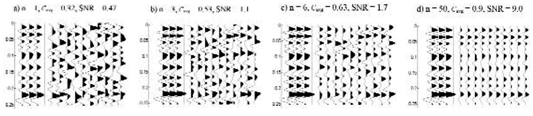
To quantify the apparent SNR of the trimmed stack, we first calculate the zero lag correlation between the individual stack traces in Figure 5, and the pilot trace, also shown in Figure 5. We then average this zero lag correlation over the 10 traces in each stacked section, and denote this average as C_avg. Clearly a C_avg of 0 would correspond to a SNR of 0, and a C_avg of 1 corresponds to a SNR of ∞. In general we write

The numerator is essentially a measure of the “signal” (or aligned noise) in the stacked traces, and the denominator is essentially a measure of their “noise” (or unaligned noise). Returning to Figure 5 we can see that the calculated SNR is roughly consistent with the displayed data. We emphasize that the “signal” in this SNR is not true signal, but is random noise aligned to mimic the pilot trace.

Variables affecting noise alignment

Figure 5 demonstrated the effect of the number of traces in a gather. Let us now consider a more complete list of variables affecting noise alignment:

• n – the number of traces in a gather
• w – the cross-correlation window, in seconds
• t_max – the maximum allowable shift, in seconds
• v – the wavelet duration, in seconds (inverse of the dominant frequency)

We will carry out several trim statics calculations for different parameter sets in order to explore the behaviour of the above variables.

C_avg dependence on w and n

In this section we establish that 1–C_avg varies as , and that w/n and t_max are variables independent of each other.

that in Figure 5, and plot various combinations of C_avg and n. From such an exercise we find that 1–C_avg vs. , yields a linear plot. Similarly, if we hold n fixed and calculate C_avg for several values of w, we can experiment and find that 1–C_avg vs. , is also linear.

In Figure 6 we combine these two trends and plot 1–C_avg vs. , where v is included to scale w to a unitless quantity. In this data, n is varying, while v = .08 and w and t_max take on fixed values for each line. (A similar graph is obtained if w is varied and v, n and t_max are held fixed in each line.)

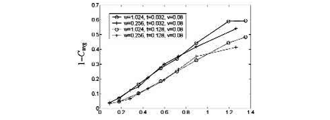
At least two aspects of Figure 6 are noteworthy. First, a linear approach to the origin is apparent both for large n and for small w. (This linearity degrades only slightly for the very largest values of n and very smallest values of w, as can be seen in the figure.) Second, the lines are grouped according to the value of t_max. This indicates that t_maxand w/n vary independently of each other.

The linear behaviour of these graphs can be readily rationalized. Allowing a non-zero t_max for random noise traces endows them with an effective non-zero signal-to-noise ratio. Noise in averaged samples generally decreases as , and this is precisely what is observed here. However, if the correlation window size is doubled, there are twice as many points to align with, and thus twice as many traces are required to produce the same result, so a w/n ratio is reasonable. At the same time, convolving with the wavelet increases the autocorrelation length from one sample to v, so (w/v)/n is also appropriate. On the basis of these plots then it seems reasonable to write the large-n, small-w limit of C_avg as

where, according to the above figures, ƒ is a decreasing function of t_max, as expected. We next delineate this function.

C_avg dependence on t_max

Can we make some guesses as to the likely form of ƒ? For a trace of random points not convolved with a wavelet, displacing a trace over an interval of [ -t_max, t_max] relative to the reference trace would be analogous to comparing the reference trace to (2t_max/dt) + 1 different traces (dt is the sample rate). Convolving with a wavelet results in an auto-correlation length of ~v, so that shifting the trace over an interval of [-t_max, t_max] would be similar to comparing the reference trace to (2t_max/dt) + 1 different traces. Thus, by analogy to the C_avg dependence on n, it is reasonable to attempt a plot of ( 1–C_avg ) vs. . This exercise is carried out in Figure 7.

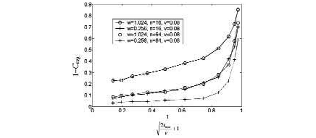
The behaviour is indeed linear for large t_max, but does not intersect closely to the origin. As expected, the lines are grouped according to their value of w/n. One could further specify Eq. (2) in its large- t_max limit as

where A and B are unknown constants, which may depend on v, but not on w or n.

A and B can be evaluated by obtaining the slope and intercept of the linear part of each line in Figure 7, and dividing those values by , then averaging the results. This gives A = 0.14±0.05 and B = 0.36±0.08 for v = 0.08s. Note that A and B are both dimensionless.

How sensitive are A and B to the value of v? We have repeated the calculation above for data obtained using v = .02s and v = .16s, with results for (A,B) of (0.21±.03, 0.38±.09) and (0.12±0.06, 0.31±0.12) respectively. From this it appears that both A and B decrease with v, but on the other hand, taking the error limits into consideration, all of the above would be consistent with A= 0.18 and any B in the range 0.29 to 0.43. We conclude that in the range of physically relevant wavelets, the dependence on v is dominated by its scaling of w and t_max, so that a convenient expression for the cross-correlation coefficient is

From the regions of Figures 6 and 7 where linear behaviour is observed to begin (and other plots not shown), we find that this expression is applicable at least for t_max > 0.06s and w/n < 0.03s, and for 0.02s < v < 0.16s.

Application to Trim Statics

Equation (4) is a key result of this paper. We will consider now how it might be employed in a practical way.

Pre-trim parameter selection

One use of Equation (4) is in choosing a set of cross-correlation parameters that will not result in significant noise alignment. In particular, one would often like to know the largest t_max that is safe to employ. Eqs (1) and (4) can be combined and rearranged to yield Eq. (5) may easily be applied to a data set. First we ascertain v, the reciprocal of the dominant frequency. Next we calculate the fold, n (which may vary from one part of the section to another). Following that we select a correlation window, and calculate its length, w. Finally we decide the upper limit of noise alignment that we will tolerate. We can do this, for instance, by considering Figure 5, where different levels of induced SNR are illustrated. From all of this information we can use

Eq. (5) to calculate the tmax that will generate this threshold SNR from pure noise. If the appearance of the resulting section reflects a much larger SNR than the designated threshold, then one may be confident that true signal has been aligned.

In Table 1 we give a sampling of t_max values obtained for various conditions. We can see that in some cases a very conservative t_max is necessary, while other data conditions tolerate a somewhat larger value. The fold appears to be a double-edged sword. We can choose a higher value of n to decrease the noise, but this increases noise alignment.

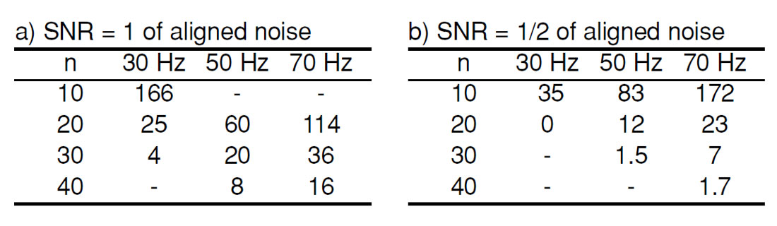
We note that the smaller t_max values become increasingly conservative, i.e. Eq. (5) gives an accurate estimate for large t_max, but too low of an estimate for small t_max (This can be deduced from the behaviour of Figure 7.) Furthermore, because Eq. (4) was derived for pure random noise, all of the t_max values are conservative in another sense as well, namely, that when true signal is present along with the noise, it will decrease the ability of the procedure to align noise. (This is illustrated in Figures 11 and 12 below.)

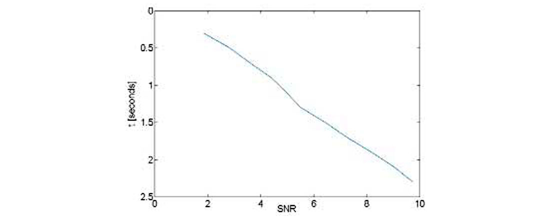
Use of Eq. (4) could have prevented the erroneous noise alignment described in the introduction. Suppose we substitute into Eq. (4) the values from the trim statics procedure of Figures 2 and 3. The window is set at 2s (between 0.3 and 2.3s) and tmax is set at 0.25s. From the frequency content v is estimated to be approximately 0.033s. Because the fold varies with depth, n is actually a function of time. It has a value of 24 at the top of the window and 280 at the bottom. Because n varies with time, so will the apparent SNR calculated from Equations (1) and (4). This result is displayed in Figure 8, which shows an estimate of SNR = 2 at the top of the window and SNR = 10 at the bottom. In Figure 9 we have taken a closer look at the portion of Figure 3 which is in the correlation window, and indeed we do see a continual improvement of resolution and decrease of noise as we move down through the window. The same is true of Figure 2 (not shown in detail).

Post-trim alignment testing

A second use of Eq. (4) is to discern after a trim statics procedure whether signal or noise has been preferentially aligned. As mentioned above, the values predicted by Eq. (4) are somewhat conservative, and one might wish to use parameters above a conservative threshold, and to tell afterward whether the choice was justified, i.e., whether signal was aligned instead of noise.

To test the utility of this method, synthetic data was created to model mixed signal and noise traces. Random noise pilot traces were created as before, but data traces for the stack were created from a mixture of the pilot trace (displaced by a static chosen from a Gaussian distribution) and an independently generated noise trace. Figure 10 shows an example of a pilot trace and a trace gather generated by static shift of each trace (but without addition yet of noise). Mathematically this is expressed as

where a_s / a_n equals the signal to noise ratio of the initial data traces. (a_n = 0 in Figure 10.) This should not be confused with the apparent SNR of the final trimmed stack, which is calculated from Eqs (1) and (4).

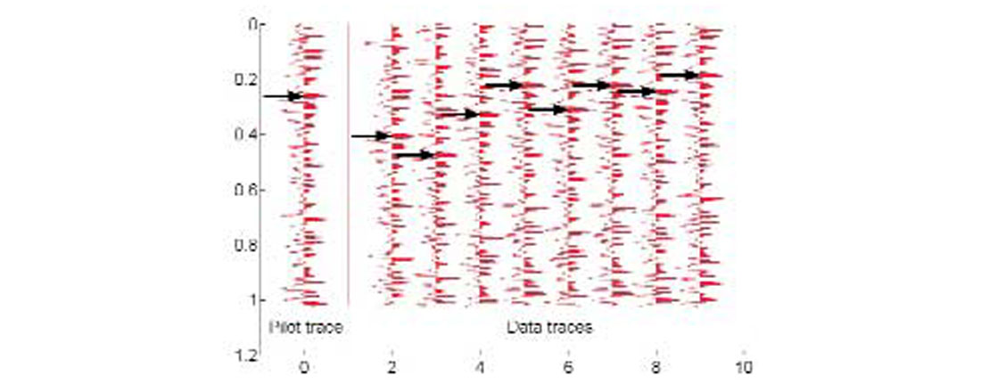
Figure 11 illustrates the t_max dependence of Cavg for three different a_s / a_n values. Figure 11a is a noisy case, in which a_s / a_n = 1/3, and the similarity of results to the prediction based on Eq. (4) suggests that noise alignment is occurring. In Figure 11b, where a_s / a_n = 2, the results level off for large t_max and are independent of w, both factors suggesting alignment of signal rather than noise. Finally, Figure 11c presents an intermediate case in which a_s / a_n = 1. Here one would conclude that the large w plots represent signal alignment, while the small w plots appear to exhibit random noise behaviour.

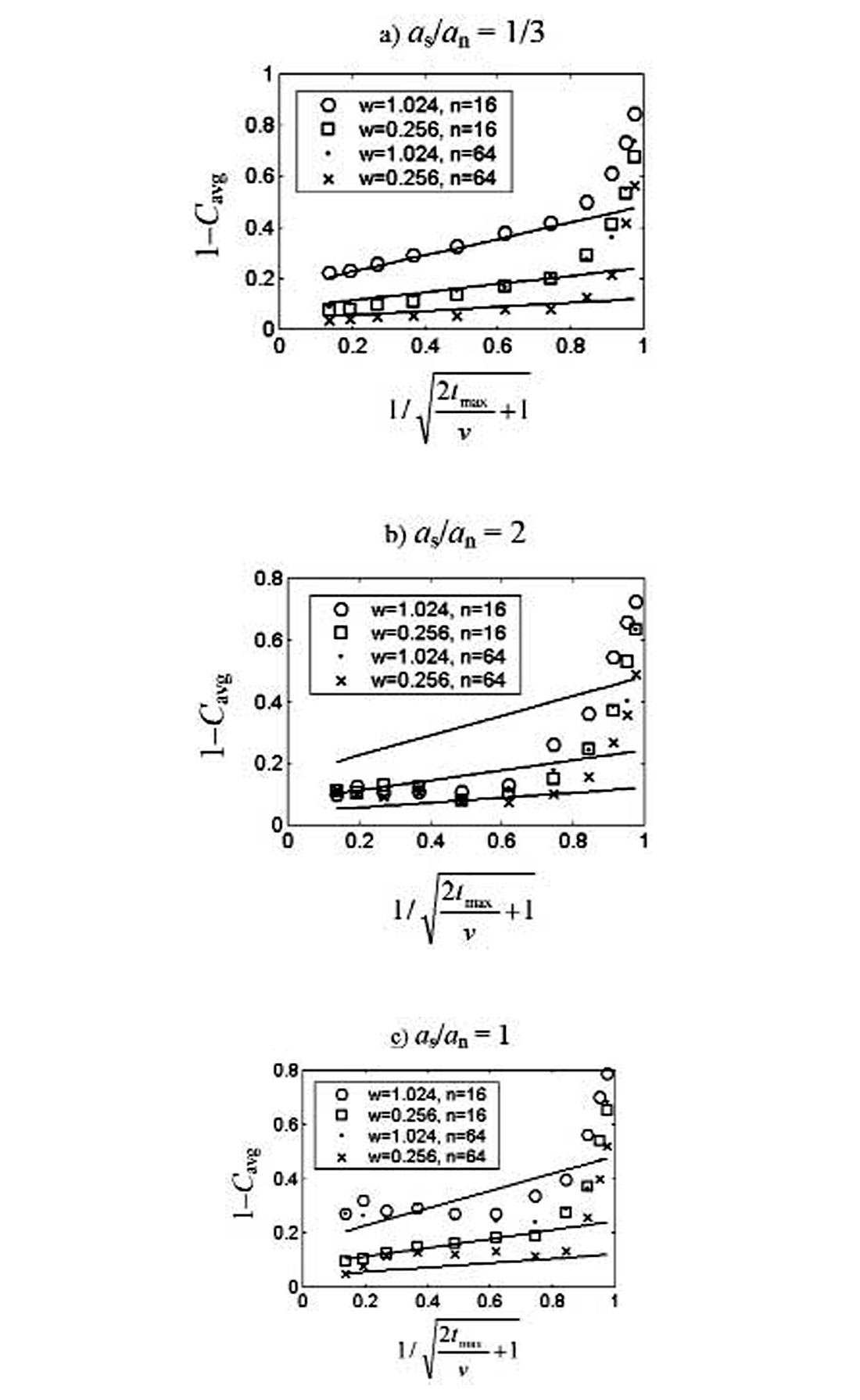
Because we have employed synthetic data, we know what shift is required for each trace in order to be aligning signal. We can use this knowledge to see whether our conclusions of noise or signal alignment in Figure 11 are correct. We have carried out this comparison and have verified that the conclusions based on Figure 11 are correct. Therefore plotting 1–C_avg against and comparing to predictions of Eq. (4) should be a valid test of noise versus signal alignment.

Another useful quantity: relative shift

In addition to C_avg, it is useful to define another quantity, the relative shift. This is essentially a comparison of realized static shifts to the maximum allowed shift. Specifically we define it as the average of the magnitude of data trace shift (t_shift ), divided by one half of the maximum allowable shift. It may be written

Dividing by tmax/2 normalizes this quantity to unity when tshift is chosen randomly from the allowed shift interval, as is the case when random noise is being aligned. This quantity can take on values between 0 and 2, but when tmax is much larger than the width of actual signal statics, the relative shift will tend to zero for properly aligned signal.

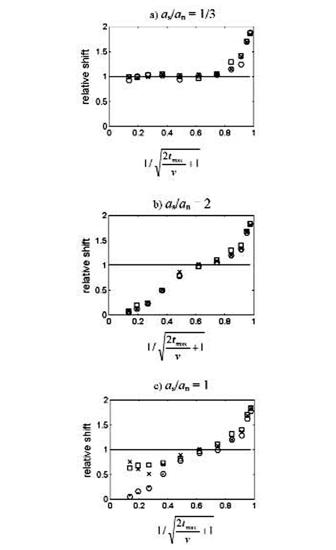
Use of the relative shift is illustrated in Figure 12, which plots information from the same trim statics calculations as in Figure 11. In Figure 12a the relative shift tends to unity. The conclusion of noise alignment in Figure 11a is thus further confirmed. Figure 12b indicates signal alignment because of the relative shift going to zero, again confirming the conclusion of Figure 11b.

In Figure 12c one would conclude that the large w plots represent signal alignment. In the small w plots the relative shift has values of <1, but are still levelling off well above zero. Apparently this trend is sufficient to imply signal alignment.

Discussion & Conclusions

In the limits of high fold, small window, and large maximum shift, the correlation procedure of trim statics is shown to be capable of aligning random noise traces to reproduce any given reference trace. The functional dependence on these parameters is shown to follow a reasonable and simple form for physically sensible frequency content, as given in Eq. (4).

This result can be of considerable practical help in choosing parameters prior to trim. To apply Eq. (4) one would only need to know w and t_max (both are input parameters), n (a property of the input data, which may also be lowered if desired), and v (a property of the input data, which may be estimated from the frequency content).

We have also shown that it is possible to determine after trim whether signal or noise has been aligned. This requires constructing trimmed stacks for several different values of t_max. From such stacks one must calculate two different quantities, which we denote as the average correlation and the relative shift. Calculation of these quantities could readily be implemented in existing trim statics calculations. Next one must examine how these two quantities vary with t_max, as illustrated in Figures 11 and 12. It appears that the average correlation is well suited to demonstrating explicitly the alignment of noise [via Eq.(4)], while the relative shift is most useful in showing conclusively the alignment of signal. Together then their characteristic behaviours should serve as useful tests in distinguishing noise alignment from signal alignment.

In cases where conventional trim parameters are suspected to be inadequate, the ideas in this paper will assist in establishing protocols for safe but aggressive trim statics.

Acknowledgements

The authors wish to thank Alan Richards for processing of the data and Alan Richards and Mike Hall for helpful discussions on this subject.