Optimization Methods for Prestack and Poststack Migration (Migration without Migraines)

Abstract

Increased efficiency of finding and developing hydrocarbon resources while reducing the environmental impact through geophysical technology is critical to the future of the petroleum industry. This technology must remotely determine rock-fluid property characteristics, their geometry, and changes over time. In reviewing advancements in exploration seismology, three component 3-D seismology stands out as the next wave and lends promise to the continued role that geophysics will play in the future of the petroleum industry.

Introduction

Recent publications continue to remind us that seismic velocity estimation remains one of the key problems in exploration geophysics. The July 1993 issue of The Leading Edge contains papers by Lines, Rahimian, Kelly, Whitmore and Garing; which emphasize the importance of velocity estimation and its relationship to the equally important problems of seismic depth imaging. For the most part, these velocity analysis methods use the prestack seismic data itself and deal with the moveout of seismic arrivals as a function of source-receiver distance. Reliable velocity estimation is seen as a necessary step in the imaging or migration process. The procedures of velocity estimation and migration become interactive in the prestack migration velocity analysis procedure. We give several model comparisons of tomography and prestack depth migration from Lines, Rahimian and Kelly (1993). These model examples correspond to similar real data examples such as shown by Lines (1991).

Poststack migration, on the other hand, does not allow for the same leverage on velocity as prestack migration but has the advantage of usually being computationally faster than prestack migration - sometimes by an order of magnitude for some problems (Johnson, 1992). Poststack migration may have inferior imaging capabilities for complex structures but may suffer less from multiple problems than prestack migration. In prestack migration analysis, velocities are computed in order to optimize some property such as focusing, or the offset consistency of depth migrations. Whitmore and Garing (1993) describe an ingenious plane wave prestack depth migration which uses the criterion that depth migrations should not depend on angles of plane wave sources. Lines, Rahimian and Kelly (1993) showed that this prestack migration method compares favorably with other velocity methods such as tomography, and is preferable for complicated structures.

It is not quite so obvious how one could optimize poststack migrations, since this process is much less sensitive to the choice of velocity functions than prestack migration. This is both an advantage and a disadvantage. It is an advantage in that the imaging is robust in poststack migration, but a disadvantage in that little information is gained concerning velocity, and reflector depths may be inaccurate. Even the prestack analysis may not help a great deal, since the stacking velocity may be difficult to interpret in terms of interval velocities. Also, the stacking velocity is derived from analysis of normal moveout. Unfortunately, anisotropy may cause NMO-derived velocities to be quite different from the velocity which is needed for conversion from time to depth.

However, the crucial velocity needed for posts tack depth migration can often be obtained from well velocity and formation depth information as derived from sonics, check shots, or VSPs. It is the purpose of this paper to briefly review optimization of prestack migration methods, and to outline a methodology for improving poststack depth migration images by the use of well information and optimization techniques.

Other methods certainly exist for using sonic velocities directly in the migration process. For example, we could attempt to smooth or "block" the sonic log in order to produce a velocity model for migration. However, there are problems in interpreting how to block the sonic or how to match sonic velocities to seismic velocities. This paper attempts a simpler approach in which a layer based velocity model will produce a migration whose depths match the formation depths from the well. This match is imposed by an iterative least squares method. Least squares was chosen due to its robustness and its ability to solve ill-posed inverse problems. In essence, this approach attempts to improve depth migration by using the formation tops to optimize our velocity estimates.

Methodology

Many excellent manuscripts have recently been written about the estimation of seismic interval velocities by optimizing prestack depth migration. In particular, the recent research of Etgen (1990), Stork (1992) and Whitmore and Garing (1993) illustrate data examples of how this can be done effectively. Generally these methods require that the velocity estimates produce prestack depth migrations which are independent of source-receiver offset.

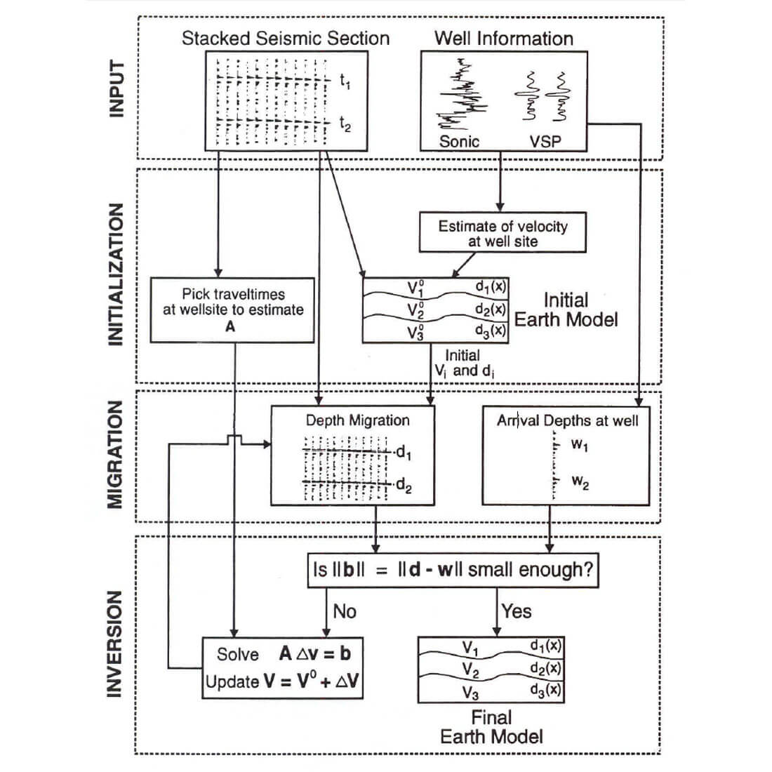
As outlined by Figure 1, our optimization methodology for post-stack migration involves the steps of data input, initialization, migration, and inversion. Input data include the stacked seismic data and well log information. From these input data, we form an initial velocity depth model in the initialization step. Seismic I-way interval traveltimes at the well site are picked for later use in the inversion process. This initial velocity model is used to perform a depth migration on the stacked data for comparison to reflector depths at the well site.

As outlined by Figure 1, our optimization methodology for post-stack migration involves the steps of data input, initialization, migration, and inversion. Input data include the stacked seismic data and well log information. From these input data, we form an initial velocity depth model in the initialization step. Seismic I-way interval traveltimes at the well site are picked for later use in the inversion process. This initial velocity model is used to perform a depth migration on the stacked data for comparison to reflector depths at the well site.

The methodology essentially requires that we minimize the sum of squares differences between the horizon depths on the migrated data d and the horizon depths from well information w.

The optimization procedure involves the use of depth migration, the development of a model from well log velocities, and the inversion for velocity which attempts to match migration depths to well log depths.

Depth Migration

The locations of seismic horizons are obtained by depth migration. One of the most general poststack depth migrations is reverse time migration which was described in a set of nearly simultaneous papers by Baysal et al. (1983), McMechan (1983) and Whitmore (1983). In this method, the time reverses of the (surface) seismic traces are the excitation functions for a wave equation finite-difference scheme which is run backwards in time. The velocities are the migration velocities, estimates of which must be known for invocation of the reverse-time algorithm. In essence, the seismic trace is propagated backward in time to the point of the "exploding reflector". In the "exploding reflector model", as introduced by Loewenthal et al. (1976), stacked seismic traces are considered to be generated by explosions initiated at time t = 0 on all reflecting boundaries and are propagated through a medium at one-half the actual seismic velocity.

The advantage of this type of algorithm is that it can use the most general wave equation modelling codes for migration purposes and is therefore not subject to the dip limitations of other migration algorithms. Despite the expense associated with reverse time migration, it is a method which provides excellent results - provided we give it an accurate velocity model.

Well Log Information

Our imaging optimization method requires that we minimize differences between seismic image depths and the depths obtained from well formation tops.

Well information may include sonic logs, formation tops deduced from cores, or vertical seismic profiles (YSP's). This information provides the necessary data, w, for our objective function, S, as defined earlier. The well data can also provide useful constraints or initial estimates in the development of a velocity model.

Optimization of Velocity from Well Information

As previously stated, our procedure seeks to minimize an objective function, S. A least squares minimization of S, as pointed out by Lines and Treitel (1984) involves the solution to sets of linear equations of the form:

Ax=b,

where x is a parameter vector whose values contain the velocity changes, A is the Jacobian matrix whose elements are given by I-way interval travel times, and b is the discrepancy vector given by

b=w-d

where w is the vector containing well depths and d is the vector containing migration depths.

It should be noted that this calculation uses an approximate Jacobian since it was derived from a flat layer model. However, Jacobian values are easily obtained by picking the seismic travel times at the well location and they may be accurate enough for us to compute a reliable inversion in a few iterations.

The optimization procedure does require some degree of interpretation in our choice of the number of velocity layers, picking the traveltimes on the stacked section, picking the depth of the migrated horizons, and picking the well formation tops. The choice of the number of layers is a problem of model parameterization which is always somewhat subjective. The picking steps are really interpretation steps to estimate A and b = W - d in the least squares equations. The computation of the depth difference, w - d, between the seismic section and the well tops can be aided by use of trace envelopes and cross-correlation methods.

Least squares is a robust method for solving the optimization problem. It is not the only method for solving the present problem.

In a well posed system, we can use back substitution to solve for the velocity change parameters.

However, if we wish to have the ability to do sensitivity analysis on the solution or solve ill-conditioned systems where the number of formation tops does not equal the number of parameters, we can resort to using least squares with a singular value decomposition solver. Let us now look at some applications of the migration and least squares inversion to a number of examples.

Applications

In order to test the effectiveness of the migration optimization method, the method was tested on models and real data sets. Model tests showed convergence of the inversion within a few (3-5) iterations.

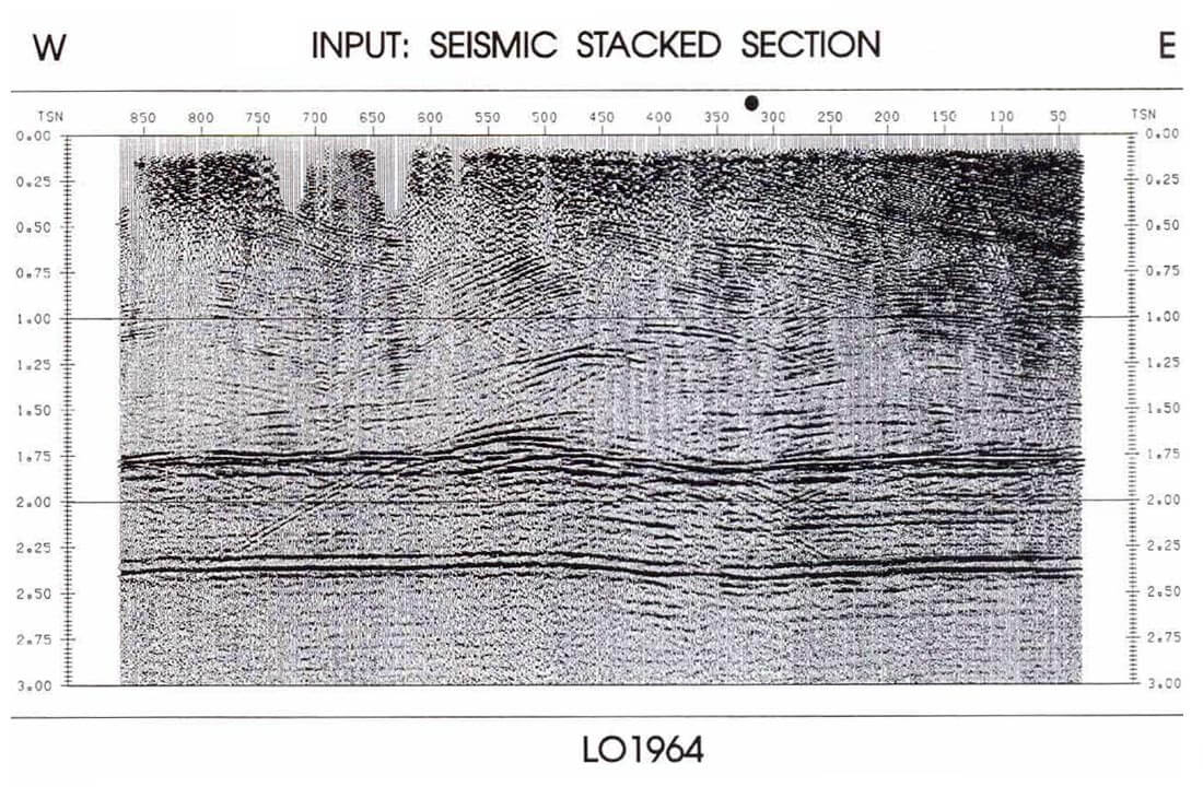
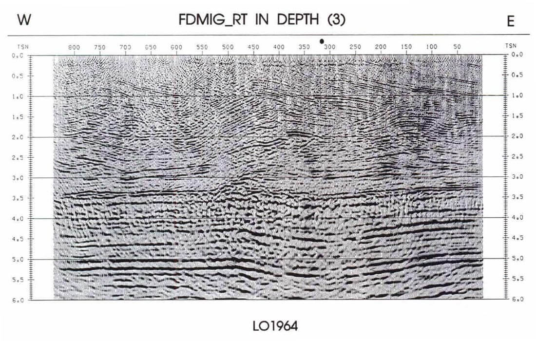
The optimized post-stack migration method was applied to real data examples. The first real data example is from the Alberta foothills, as supplied by Lithoprobe and Gulf Canada. The original stacked data of Figure 2a shows that the interpretation would be obscured by a series of diffraction hyperbolae for events between 1.0 and 2.0 seconds in the middle of the seismic section. The application of reverse-time finite-difference depth migration with the previously described optimization procedure produces the depth migration of Figure 2b which is a much more interpretable depth image. The average error in the formation depth is about 40 m, or less than 1/2 of a wavelength. The initial result produced by velocity estimates based on the sonic provided a good image in the first iteration and the improvements with later iterations were incremental. In summary, the image produced by the optimization procedure produced an encouraging result.

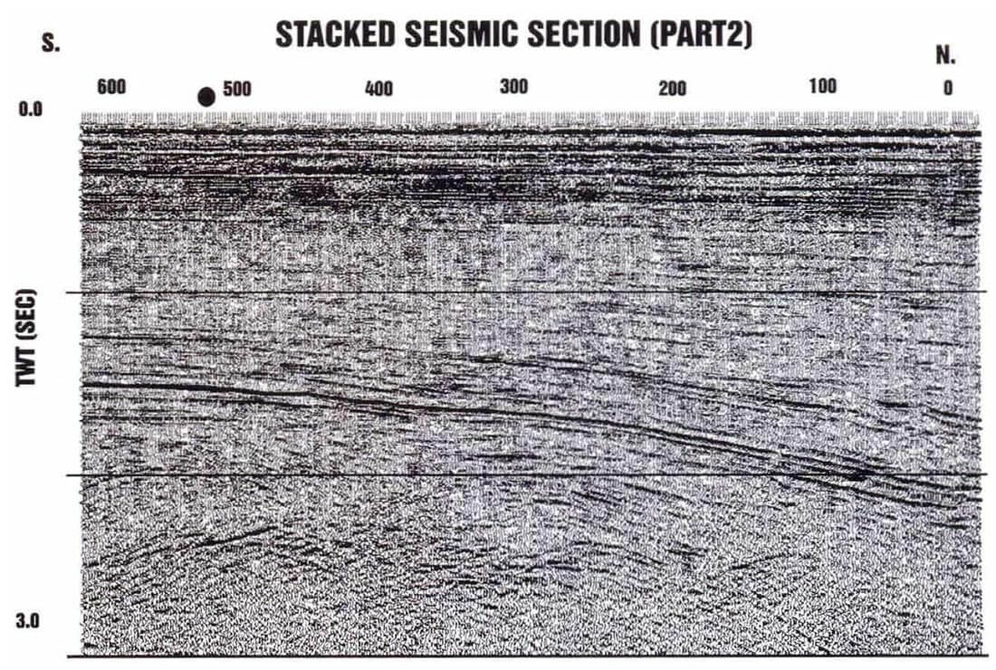
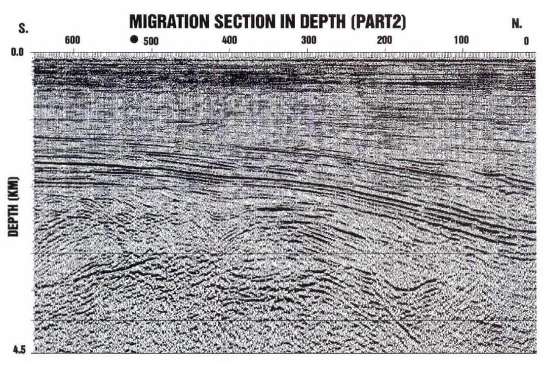
The final example shown here is from offshore Newfoundland. The input stacked time section in Figure 3a does not show clear definition of Cretaceous and Jurassic sediments below 2.0 sec. The depth migration of Figure 3b shows a more clear image of these sediments which are at depth below 2.5 km. A syncline below S.P.200 at a depth of 3.5 is much clearer on the migration of Figure 3b than in Figure 3a. Optimization of migration generally reduced average depth errors of 30m to 10m or less. Basically the migration improvements are incremental but worthwhile.

Conclusions

Poststack depth migration with the finite-difference reverse-time algorithm is a robust method of seismic imaging. However, unlike prestack migration methods, the method gives little information about seismic interval velocities. If well data are available, these problems of depth imaging can be obviated by using well information to optimize post-stack depth migration. The feasibility of this method is demonstrated by use of synthetic and real data examples. Although this paper shows only a few examples, the results are encouraging. It is our intention to share these ideas of optimizing migration in order that the method can be tested further on several data cases.

Acknowledgements

The funding for this research was made available by Natural Sciences and Engineering Research Council of Canada and by Petro-Canada Inc. Their support is gratefully acknowledged. Also, the authors wish to thank Tony Kocurko for his valuable support of the computer systems utilized in this project. We also thank Theresa Lannan and Shirley McLaren for their word processing and drafting assistance. A Fortran version of Golub and Reinsch's "minfit" program was generously provided to us by Freeman Gilbert of Scripps Institute of Oceanography. The real data set from Alberta foothills was provided by Kris Vasudevan of Lithoprobe and John Pendrel of Gulf Canada and the offshore Newfoundland example was provided by Gary Taylor of Hibernia Management and Development Corporation. Finally, we thank David Eaton, Sam Gray, Fred Hilterman, Don Lawton and Sven Treitel for their constructive comments on the manuscript.