On Hookean solids in seismology: anisotropy and fractures

1. INTRODUCTION

Geophysics—similarly to astrophysics—relies on remote sensing. Inferring material properties of the Earth’s interior is akin to inferring the composition of a distant star. In both cases, scientists rely on matching theoretical predictions or explanations with observations. Notably, obtaining a sample of a material from the interior of our planet might not be less difficult than obtaining a sample from a distant celestial object.

To infer the presence and orientations of subsurface fractures, seismologists might use directional properties of Hookean solids. In other words—using such a solid as a mathematical model— seismologists match its quantitative predictions with observations.

A Hookean solid is a mathematical entity. It is defined as an object, c_ijkℓ , that relates stress, σ_ij , and strain, ε_kℓ , in a linear fashion; this relationship is called Hooke’s law. c_ijkℓ shares the Platonic realm with its other occupants, such as a point, a sphere, an equation. Also, it appears to provide fruitful analogies to examine quantitatively physical phenomena.

When invoking Platonic analogies, which is a common method in physics, we must be aware of their limitations. To say that P and S waves are two types of disturbances that propagate in the Earth is a shorthand for saying that if we use an isotropic Hookean solid as an analogy for the material of our planet, then we can associate disturbances in the Earth with the wave equations in such a solid. While these disturbances result in detectable phenomena, the wave equations have solutions, which might be used as quantitative analogies to study these phenomena.

The subject of this article is a connection between detectable phenomena and mathematical entities used as their analogies, in particular, between the effect of fractures on seismic disturbances and the effect of anisotropy on waves in Hookean solids, which is a connection between properties of rocks and symmetries of tensors. The motivation for this article is to gain an insight into issues of which we might not be aware if our familiarity with the subject comes mostly from applications. We might not entertain doubts and, hence, not pose questions that should accompany applications. In the following quotation, Charles Sanders Peirce [12] warns us about this mistake.

Persons who know science chiefly by its results […] are apt to acquire the notion that […] it is only here and there that the fabric of scientific knowledge betrays any rents.

We begin this article by discussing symmetries of Hookean solids and their analogies to fractures and layering. For instance, disturbances in layered rocks lend themselves to an analogy of waves in anisotropic Hookean solids. Then, we discuss the concept of precision and accuracy in the context of these symmetries. We conclude this article by discussing inferences of material properties from seismic measurements with errors.

Even though this article deals with mathematical concepts, we discuss explicitly only a few mathematical operations. Nevertheless, we strive to maintain the rigour of statements, and we refer readers to specific papers for further details. For instance, the proof of the aforementioned relation between parallel isotropic layers and anisotropy is formulated by Backus [2].

2. SYMMETRIES

The concept of symmetry is one of the most important notions of mathematics and physics. For instance, as shown by Emmy Noether [11] a century ago, all conservation laws are expressions of symmetry. Notably, the ray parameter is a conserved quantity that is a consequence of a translational symmetry intrinsic to parallel layers.

In this section, we focus our attention on rotational symmetries of Hookean solids, which is the subject of anisotropy. Since these solids are mathematical entities, we must describe such a symmetry as a mathematical concept.

In a manner similar to the everyday meaning of the word, mathematical symmetries mean that we can perform operations on an object without modifying its appearance. A sphere can be rotated by any amount about any axis without changing its appearance. Likewise, wave-propagation properties within an isotropic Hookean solid are independent of its orientation, giving them spherical symmetry. We might expect that such a behavior is a good analogy for granites, which exhibit a random arrangement of quartz, mica and feldspar, but not for shales, where properties of disturbances propagating along laminations might be quite different from properties of disturbances propagating obliquely to laminations.

Even though, heuristically, a Hookean solid could be illustrated as an idealized physical object, it is no more and no less than a tensor, which exists in the realm of mathematics only. Hence, its symmetry is only a mathematical property: an operation that leaves this tensor unchanged. We can exemplify it by rotating a second-rank tensor in two dimensions, whose components, α_ij , can be written as a 2 × 2 matrix. The condition of symmetry is

where T denotes transpose. In other words, we ask for the values of α_ij that leave this tensor unchanged for a given angle θ. It can be easily shown that if α₁₁ = α₂₂ and α₁₂ = α₂₁ = 0 , the tensor is isotropic: it remains unchanged for all angles. Also, if θ = π , the matrix remains unchanged for any values of α_ij . This is a consequence of the so-called point symmetry, which is invariance to the action of the negative identity, −I ; geometrically, it means that properties are sensitive to direction but not to the sense; it does not matter if we go NW or SE as long as we remain on a NW-SE line. Notably, all even-rank tensors, which includes Hookean solids, exhibit that property. Used in seismology, this property implies that velocity, which might depend on direction, does not depend on the sense. Herein, the point symmetry is also the twofold symmetry, which—according to Herman’s Theorem [9]—is the highest discrete symmetry that a second-rank tensor can have. Notably, Hookean solids, which are fourth-rank tensors, cijk_ , can have up to the fourfold symmetry, but not beyond.

Let us use the above example to gain an insight into limitations of tensors as analogies for quantifying physical properties. Using aij , we cannot distinguish among objects whose discrete symmetries are twofold, threefold, fourfold, etc., since invariance under any rotation implies isotropy. Consider, for instance, a fourfold rotation, which means that θ = π/2 . In such a case, the symmetry condition becomes

To satisfy this condition, we require that α₁₁ = α₂₂ and α₁₂ = α₂₁ = 0 , which—as stated above—is tantamount to isotropy. Also—due to point symmetry—we cannot study phenomena for which properties depend To satisfy this condition, we require that α₁₁ = α₂₂ and α₁₂ = α₂₁ = 0 , which—as stated above—is tantamount to isotropy. Also—due to point symmetry—we cannot study phenomena for which properties depend on going left versus going right along a given direction. Thus the analogies provided by a second-rank tensor in two dimensions are limited.

We can distinguish between isotropy, which is the invariance of properties under any rotation, and anisotropy, which is the sensitivity to any rotation, except—due to the point symmetry—the rotation by π.

Since Hookean solids are fourth-rank tensors, c_ijkℓ , the analogies they provide are richer than analogies provided by the second-rank tensors, α_ij ; nevertheless, they are limited. Let us name a few limitations. The fourth-rank tensors cannot have two orthogonal symmetry planes only, since their even rank implies that they can have either a single symmetry plane or three symmetry planes. This statement does not mean that rocks themselves cannot exhibit only two sets of planar features that are orthogonal to one another; an example of such an arrangement is parallel layers with a set of parallel fractures perpendicular to these layers. It means, however, that such a physical arrangement does not have a direct symmetry-class analogy among Hookean solids. For such an arrangement, the Hookean analogy has three orthogonal symmetry planes; two of them are direct analogies of fractures and layers; the third one is a byproduct of mathematical properties of the even-rank tensor. While it is not uncommon to obtain—as a mathematical byproduct—nonphysical solutions, which can be subsequently rejected, in the case of the Hookean analogies, we cannot distinguish if a three-plane model is an analogy for two or for three sets of planar features; both are physically possible.

Another limitation is the fact that—while we can distinguish among the twofold, threefold and fourfold symmetries—we cannot distinguish among discrete rotational symmetries beyond fourfold. Hence, there are no pentagonal or hexagonal classes for Hookean solids; as proven by Herman [9], all rotational symmetries higher than fourfold possess transverse isotropy. Even though the importance of crystallography in studies of symmetries led to the borrowing of its nomenclature, this resulted in misleading terminology for continua. For instance, the hexagonal symmetry is an inappropriate term for Hookean solids, even though we might infer it from tessellation … but that could be a subject of another article.

Symmetries of tensors are distinct from lattice symmetries, which means that we must not be hasty with comparisons between symmetries of Hookean solids and symmetries of crystals. For instance, the former allow for continuous symmetry groups, namely, isotropy and transverse isotropy, and the latter allow for discrete symmetries only. The above distinction stems from the essence of continuum mechanics, where we describe properties of materials by continuous functions, not by considering discrete structures. This statement does not contradict the fact that symmetries of continua serve as analogies for such structures as fractures within materials.

Let us complete this section by emphasizing that—while using seismic information—we must remember that seismology is a subject of continuum mechanics. As stated by Aki and Richards [1],

there is a conjecture that two sets of small motions may be superimposed without interfering with each other in a nonlinear fashion. … These conjectures, and many others that are generally assumed by seismologists to be true, are properties of infinitesimal motion in classical continuum mechanics.

3. ACCURACY

Since a theory is unavoidable to mediate between measurements and interpretations, let us examine—within such a theory—the accuracy of representing a generally anisotropic tensor, inferred from physical measurements, by its more symmetric counterpart.

Prior to that examination, let us acknowledge an abuse of terminology. Below, we consider the components of the elasticity tensor, to which we refer as the elasticity parameters, and their standard deviations. Since the elasticity tensor is not the object of measurements, but a mathematical entity inferred from them, it is nonsensical to discuss whether or not the tensor is accurately measured. Herein, given the tensor components with their standard deviations—and remaining within the realm of mathematics—we discuss the accuracy with which this generally anisotropic tensor is represented by its symmetric counterpart to which we refer as its effective tensor. There are two other aspects of accuracy. First, the generally anisotropic tensor is obtained, through an inverse theory, from seismic measurements. Hence, we could attempt to relate its standard deviations to measurement errors. Secondly, once the effective tensor is chosen, we could examine the accuracy that it provides for modeling physical phenomena. Neither issue is the explicit subject of our discussion. Thus, aware of these subtleties, we use the meaning of accuracy and precision sensu lato.

In a manner similar to the statement about the P and S waves propagating in the Earth, discussed above, the statement that a material is transversely isotropic is indirect. It means that properties of waves in a transversely isotropic Hookean solid allow for sufficiently accurate descriptions of waves in a generally anisotropic continuum, and— subsequently—that waves in such a solid are accurate analogies for propagation of disturbances in the material whose measurements resulted originally in the generally anisotropic tensor. In our subsequent discussion, we mean the above sequence of statements when we say, as a shorthand, that a given symmetry and orientation of a tensor is an accurate analogy for the material in question.

To examine materials in terms of Hookean solids, which are fourth-rank tensors expressed in terms of twenty-one independent components, we make measurements that allow us to estimate these twenty-one components; it is not an easy task … and again it could be a subject of another article. The importance of all twenty-one components is the fact that, as shown by Bóna et al. [3], they contain implicitly the information about the orientation of the tensor. Consequently, it is not necessary to assume a priori, as is the case if we consider ab initio particular symmetry classes, that we deal with, say, the transverse isotropy with the vertical symmetry axis.

Dewangan and Grechka [8] obtained the twenty-one components from vertical-seismic-profile measurements in New Mexico. Their estimate is

which are the density-scaled elasticity parameters, whose units are km²/s².

Once these parameters are estimated, we can proceed to find the symmetry class and orientation of the tensor that is the best analogy for the rock subjected to seismic measurements. Such a symmetry allows us to interpret features of the material in question. For instance, a monoclinic symmetry is consistent with obliquely fractured parallel layers, as described by Winterstein [17].

We must quantify the meaning of the best analogy in the context of the precision with which the generally anisotropic tensor is given. To do so, we invoke the concept of proximity, which allows us to say that the closest analogy that is consistent with our material is, say, a monoclinic Hookean solid with a dipping symmetry plane. In turn, to quantify the concept of proximity, we must define the notion of a distance among fourth-rank tensors. Two distinct norms appear to be of particular interest in seismology, the Frobenius norm and the L₂ norm . . . but again, let us postpone such a discussion for another article.

Once we establish the tensor of a given symmetry that is closest to the twenty-one parameters obtained from the measurements, we can examine whether or not this tensor can be used as an effective counterpart for the generally anisotropic Hookean solid, in the context of the standard deviations of that tensor. The higher the symmetry of a given Hookean solid, the further it is from the generally anisotropic Hookean solid; hence, isotropy is the most distant model.

In the case of isotropy, the twenty-one parameters are reduced to two, which are referred to commonly as the Lamé parameters, λ and µ . For instance, about a century ago, Voigt [15] showed that the closest isotropic solid—in the Frobenius sense—is

and

where

and

Herein, c_ijkℓ are the components of the generally anisotropic Hookean solid;

and

are the components of its closest isotropic counterpart.

From the fact that the higher the symmetry of a given Hookean solid, the further it is from the generally anisotropic Hookean solid, it follows that the closest counterpart is necessarily the least symmetric tensor. However, the effective tensor is not the closest one, but the most symmetric one, which means the furthest that is acceptable within the precision with which the twenty-one parameters are given. This is an epistemological, as opposed to ontological, statement of Occam’s Razor; we do not claim Nature’s propensity for simplicity, we just recognize our limitations in analyzing her complexities. Let us examine that issue.

Dewangan and Grechka [8] include the following standard deviations with their estimate of twenty-one parameters:

Considering these standard deviations, we view the parameters of the effective tensors not as specific values but as ranges within which lie the best-fit values. To obtain these ranges, we follow the Monte-Carlo method (e.g., Tarantola [13]).

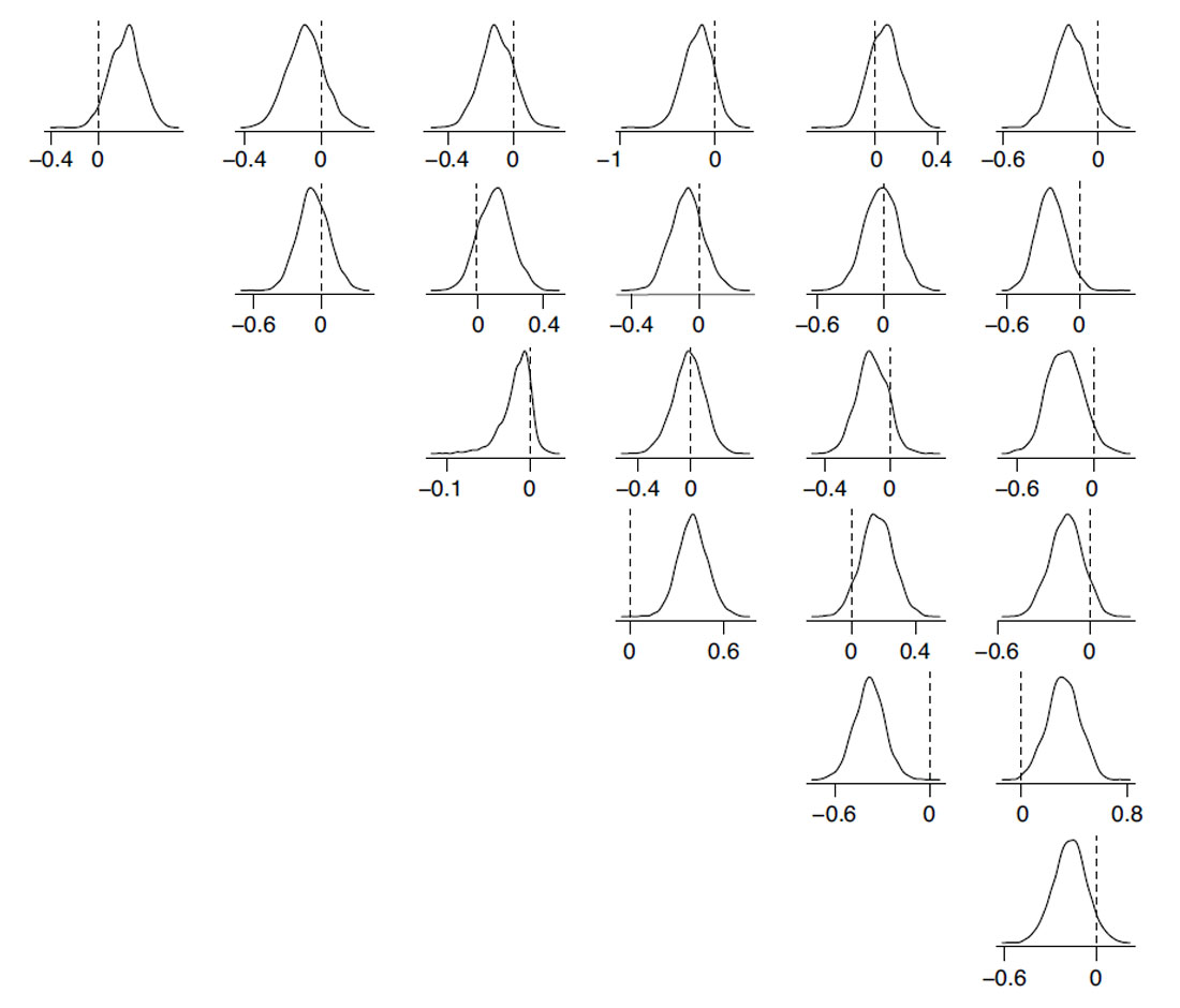
To find the symmetry class of the effective tensor, not to be confused with the closest symmetry class, which is necessarily the least symmetric, we require the most symmetric tensor such that the difference between that tensor and the generally anisotropic one be contained sufficiently within the error ranges of the elasticity parameters of the latter. For instance, considering the transversely isotropic tensor, we obtain—for each of the twenty-one parameters—the empirical distribution of the differences between the components of the generally anisotropic and symmetric tensors. Examining the histograms in Figure 1, we might conclude that the transversely isotropic Hookean solid is not a good enough analogy for the material examined by Dewangan and Grechka [8]. Were it a good analogy, most zero differences would be close to the centers of the histograms.

To illustrate quantitatively this condition, let us consider the highest symmetry: isotropy, for which the effective tensor is independent of orientation, and—unlike for other symmetry classes—for all orientations, all

except

and

Using the twenty-one parameters obtained by Dewangan and Grechka [8], we can find the closest isotropic tensor by invoking Voigt’s [15] formulas. The question, however, remains: is it a good enough analogy for the physical material under consideration? To shed light on this issue, let us consider the entries that are zero. The entry at the first row and the fourth column is 0.1374 ± 0.1176 , which means that zero is more than one standard deviation away; it follows from properties of the Gaussian distribution that probability of the required zero is less than 30% . For the entry at the second row and the sixth column, 0.1692 ± 0.0832 , the required zero is more than two standard deviations away; its probability is less than 5% . Thus, conditions for isotropy are not likely to be satisfied.

The fact that there is no orientation dependence renders the problem of finding the effective isotropic tensor much easier than for other classes. The need to involve rotations in the search for the other effective tensors leads to a highly nonlinear problem, which requires advanced numerical techniques as discussed by Kochetov and Slawinski [10] and Danek et al. [7]; this is the reason why, a century ago, Voigt [15] formulated the closest tensor for isotropy only; he was aware of limitations of computational methods at his disposal. Also, in the isotropic case, we can consider analytically the concept of normal distributions and standard deviations. For other cases, we need to study the error propagation numerically—by such approaches as the Monte-Carlo method—to obtain empirical distributions.

However, in pursuing computational methods, Kochetov and Slawinski [10] and Danek et al. [7] base their formulations on the fundamentals of continuum mechanics and obtain the solutions for the resulting equations by analytical methods, if possible. Thus, they are mindful of, and share the concern with, Weglein [16] who writes that

the need for ever-faster computers is universally recognized and supported. However, the growth in computational physics, often at the expense of mathematical physics, and the availability of ever-faster computers, encourages the rush to “cost functions” and to searching without thinking, and thus represents a ubiquitous, misguided, and unfortunate trend, with “solutions” that are not.

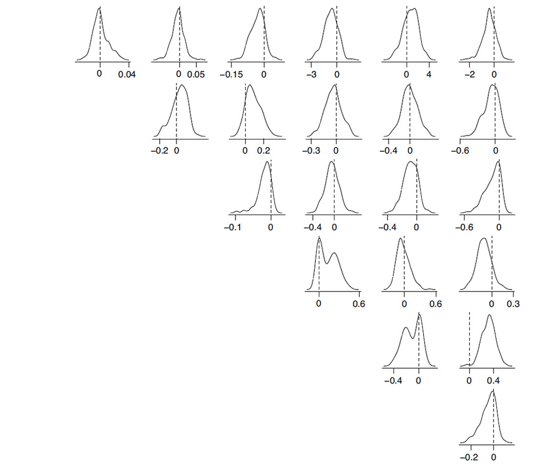
As discussed by Dewangan and Grechka [8] in their original study, and subsequently by Danek and Slawinski [6], Kochetov and Slawinski [10] and Tsvankin and Grechka [14], the orthotropic symmetry, which is less symmetric than transverse isotropy, appears to be a good analogy for the twenty-one parameters and their errors, as illustrated by histograms in Figure 2. Comparing Figures 1 and 2, we see that the zero differences between the parameters of the generally anisotropic Hookean solid and the parameters of its symmetric counterpart are contained better within histograms of the latter case.

We strive to ensure that our inferences are justifiable by accuracy of the generally anisotropic tensor. In general, the higher the symmetry, the simpler the model; an isotropic Hookean solid contains less information than any solid of lesser symmetry. To invoke a less symmetric analogy, we need more information, such as a sufficient resolution to distinguish among the elasticity parameters. Consequently, proposing an isotropic model might be a statement about intrinsic properties of the material in question or it might be a statement about the limited accuracy or precision. In the present example, it is sufficiently high to consider an analogy not with two values, which describe isotropy, but with twelve values: nine elasticity parameters describing properties of an orthotropic Hookean solid and three angles describing orientations of its symmetry planes.

4. INFERENCES

Seismologists who infer material properties from observed seismic phenomena are implicitly or explicitly concerned with inverse problems. Such inferences are inductive, not deductive, processes, even though quantitative seismology is formulated from axioms by a deductive process; for instance, the existence of the P and S waves is deduced from the balance of linear momentum in a Hookean solid. As Peirce states laconically in 1908,

Deduction [and] induction […] render the indefinite definite; deduction explicates, induction evaluates: that is all.

Backus [2] uses deduction within the realm of Hookean solids to explain how anisotropy is produced by layering. Data that appear to be consistent with such an anisotropy might allow us to evaluate the layered composition. Given the axioms, the former is certain; the latter is an interpretation.

Let us consider several cases. An accurate enough analogy of a seismic behavior with a model of a transversely isotropic Hookean solid is consistent with parallel layers. An accurate enough analogy of a seismic behavior with an orthotropic solid is consistent with parallel layers and a perpendicular set of parallel fractures. An accurate enough analogy of a seismic behavior with a monoclinic solid is consistent with parallel layers and an oblique set of parallel fractures. However, none of these cases is the only possible interpretation, and the choice of a preferred interpretation might rely on information beyond seismic anisotropy.

Let us emphasize that the analogy between the anisotropy and layers or the anisotropy and fractures relies on the assumption that the thicknesses of parallel layers or the separations between parallel fractures are much smaller than the wavelength used for their examination. Heuristically, we could view the passage of such a wave as a process of averaging over a wavelength the properties of discrete objects for which the anisotropy might serve as an accurate-enough analogy within the realm of continuum mechanics. Anisotropy, on the other hand, is a property of a continuum, and as such—by the definition of a continuum—it is scale independent: a continuum exhibits the same macroscopic and microscopic properties. Thus, the same continuum with its anisotropy might serve as an analogy for the behavior of waves both in a crystal and in a sedimentary basin.

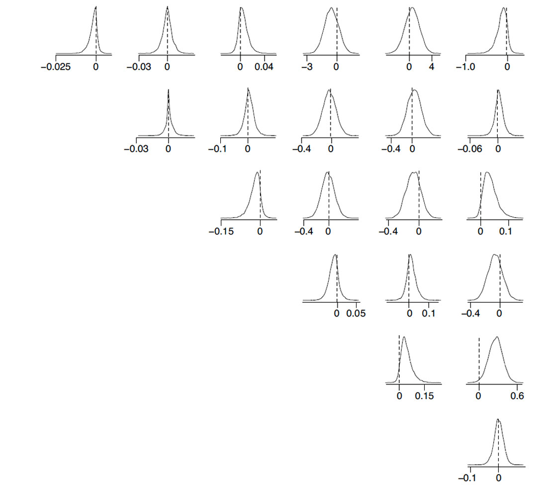
Furthermore, the intricacies of accurate enough must be understood. Examining Figures 1, 2 and 3, we see that the choice of a model itself is not obvious since, necessarily, the less symmetric the model, the better its fit. Figure 3 exhibits a better fit than Figure 2, which in turn exhibits a better fit than Figure 1. We do not need to generate histograms to know that the most accurate analogy is provided by a generally anisotropic Hookean solid. However, achieving the best fit is not our purpose. If we wish to gain an insight into directional patterns in the subsurface, we must consider symmetric Hookean solids— rather than a general one, which is consistent with the randomness of layers, fractures or grains—at the expense of accuracy. Thus, we need criteria other than the fit itself; for instance, a criterion that examines the increase in accuracy as a function of the number of parameters. The transversely isotropic model has seven parameters, which are five elasticity parameters to describe elastic properties and two Euler angles to describe orientation of the symmetry axis; the orthotropic model has twelve parameters; the monoclinic model has fifteen parameters. To answer quantitatively whether or not the increase in the number of parameters is justified by the improvement of the fit, we might consider information criteria, such as the Bayesian analysis, … but yet again, let us postpone this discussion for another article.

Also, let us mention that even perfect knowledge of the wavefront symmetries is insufficient to infer the material symmetry. According to Curie’s Principle [5], the symmetries of the causes must be found in their effects, but the converse is not true; that is, the effects can be more symmetric than the causes. In other words, Hookean solids can be less symmetric than wavefronts within them. However, Bóna et al. [4] show that we can determine the symmetries of the solid if we combine the information about the symmetries of wavefronts and about symmetries of polarizations.

5. CONCLUSIONS

Since in seismology we use remote measurements—such as geophones on the surface responding to disturbances within the interior—the inferences between the measurements and the properties of the interior, such as fractures, must be mediated by a theory. For seismology, this theory is continuum mechanics. For better or worse, seismologists are confined to having an intermediate step between measurements and information about properties of the zones of interest. In inferring material properties from mathematical models, the best we can do is to achieve consistency between model predictions and observations. For instance, my not receiving answers to letters sent to Robert Hooke is consistent with his being dead, but it does not entail it. If I have no information beyond my epistolary attempts, a possible—and perhaps likely—interpretation is his not being interested in correspondence with me. As emphasized by Tarantola [13], we can infer properties from models by induction, not deduction.

The emphasis of this article consists of three points. First, anisotropy considered in the context of seismic measurements is a mathematical analogy for physical properties of materials. It deals directly with the symmetry of tensors and only indirectly with material properties of rocks. Secondly, the interpretation begins with the choice of analogy, as illustrated in discussions of Figures 1–3, where the choice depends on the concept of sufficient accuracy with which a symmetric tensor represents the generally anisotropic one. Thirdly, once the analogy is chosen, there are many physical situations that can account for that analogy. Anisotropy of a Hookean solid implies—by analogy—a directional pattern within a material, as opposed to, say, a random arrangement. However, it does not provide explicit information about the causes for a given pattern or its absence. Transverse isotropy might be an analogy for parallel layers in a sedimentary basin or for the preferred orientation of olivine crystals in the Earth’s mantle.

Thus, the relations between anisotropy and fractures, while containing insights into material properties, must be applied with awareness of their limitations. Among pertinent questions there should be an inquiry into criteria for the choice of a model. We should be aware of the extent to which the model itself is imposed. For instance, is the model with the transverse isotropy whose symmetry axis is vertical imposed a priori, and if so have the observations been forced into a model that is not optimal? Just as many physical scenarios can be proposed to accommodate a given model, many models can be proposed to accommodate experimental data, particularly, if errors are taken into account. Herein, in the discussed approach, where the original information is taken from a generally anisotropic tensor, the orientation is implicitly contained within its twenty-one components; hence, not only the elasticity parameters, but also the orientation of the symmetry axis is obtained directly as an inverse solution. Thus, recognizing the advice of Weglein [16] who refers to the indirect model-matching methods, and according to whom

[m]athematicians […] would better spend their time describing the underlying lack of a necessary and sufficient condition, and the consequences,

the discussed approach relies on the direct solutions formulated by Bóna et al. [3].

In conclusion, the awareness of the necessity for a theory to mediate between measurements and interpretations—and hence the unavoidable presence of abstract concepts, such as symmetry of tensors, for analysis of physical properties, such as fractures—is crucial for applied geophysics, as, in general, is the awareness of pitfalls in using any theory to explain, interpret or predict physical phenomena.

Acknowledgements

The author wishes to thank Rob Kendall for suggesting this article, following the seminar in honor of Tadeusz Ulrych, and to John Fernando for his editorial support. Also, the author wishes to acknowledge numerical analysis of Tomasz Danek and editorial work of David Dalton and Elena Patarini, as well as discussions with Tomasz Danek, Ayiaz Kaderali, Roger Mason, Ilya Tsvankin and Art Weglein.

This work was performed in the context of The Geomechanics Project supported by Husky Energy and the Natural Sciences and Engineering Research Council of Canada.