There have been several comparisons of Mega-Bin and orthogonal 3D seismic survey designs over the years. In this paper, we demonstrate a different way to normalize the two types of surveys by creating each design so as to have identical field acquisition efforts and costs. From this vantage point the trace statistics for each survey are better compared. It becomes evident that some advantages that were attributed to the Mega-Bin design when employing post-stack migration may no longer be advantageous when using 5D regularization, multi-channel pre-stack noise attenuation in multiple domains, and PSTM.
Method
The basic requirements for imaging the reservoir of interest were established using typical 3D seismic survey analysis (for example, Cooper 2004). Existing seismic data in the area were analyzed for signal and noise properties. The target reservoir structure and required vertical/horizontal resolution were considered and pre/post-stack pay zone signatures were modeled. The resulting data requirements are summarized in Table 1.
| Table 1 | |
| Maximum usable source to receiver offset | 775 metres |
| Desired offset with 360° azimuths | 775 metres |
| Maximum subsurface bin size | 30 metres |
| Trace density required at 775 meter limit | 18,000 trace/km2 |
| Surface area | 6 km2 |
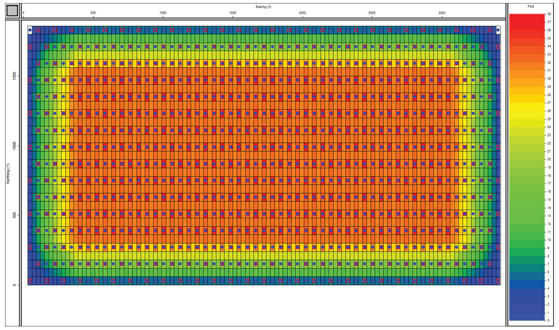
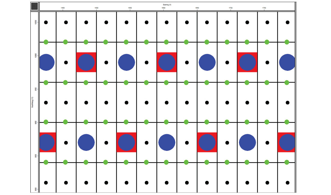
A nearby existing Mega-Bin survey satisfied all of these requirements. It consisted of 120 metre receiver line spacing with 60 metre receiver intervals and a coincident source point on every second station. A 6 km2 pre-plot design with this source and receiver layout is shown in Figure 1.
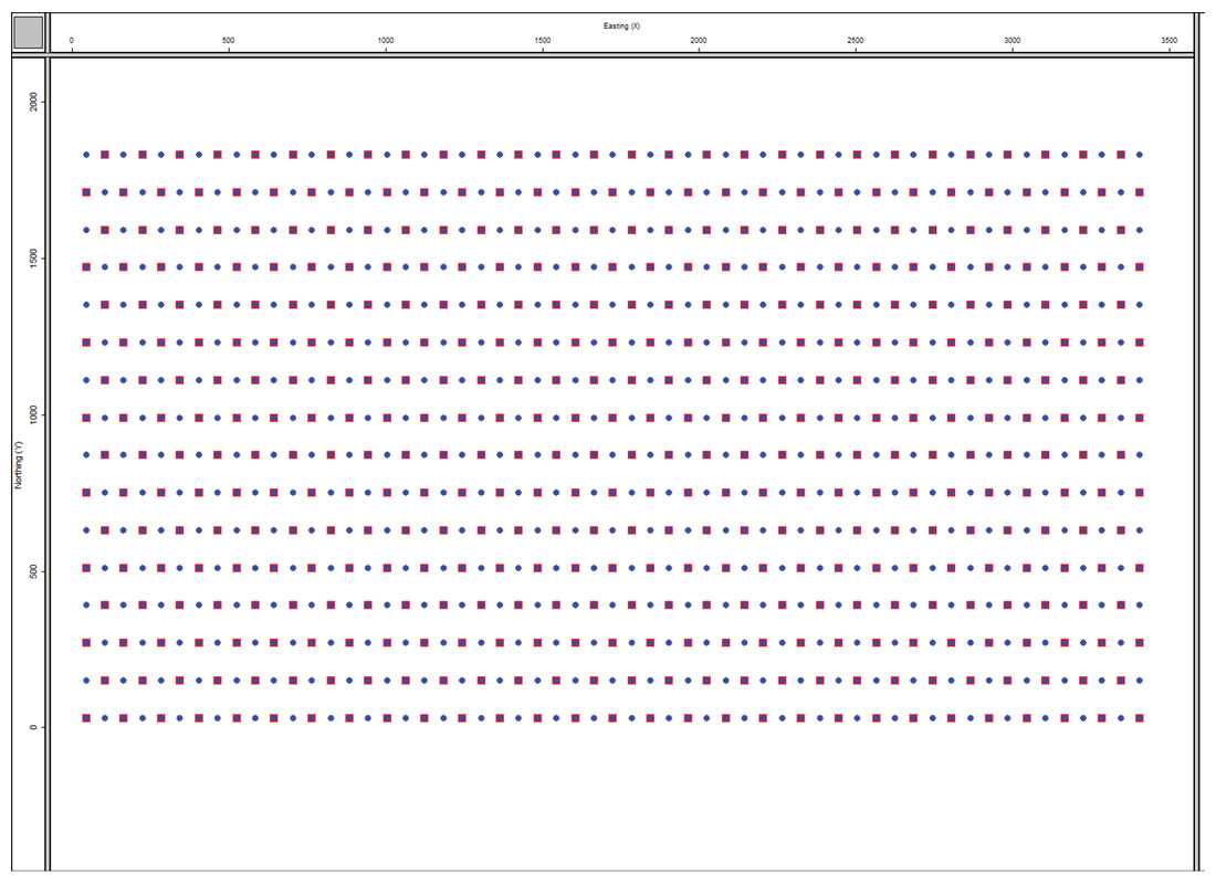
The set-up in Figure 1 is standard Mega-Bin design and conforms to the requirement of the patent that the sources are coincident on the receiver stations (Goodway 1996). Field logistics would probably result in recording the survey with all channels live. However, the data analysis showed that seismic data recorded with greater than 775 metres to receiver offset does not contribute to the zone of interest imaging. The operational statistics which determine the cost of acquisition are listed on the left side of Table 2.
It should be noted that the natural bin size for this Mega-Bin survey is 30 x 60 metres which violates one of the survey requirements. Since the Mega-Bin inception it has been expected that interpolation will be used in the direction of the coarsest spacing, which is in the cross-line direction (Goodway 1996, Goodway 2012). This interpolation step resulted in 30 x 30 metre bins thereby meeting that design requirement.
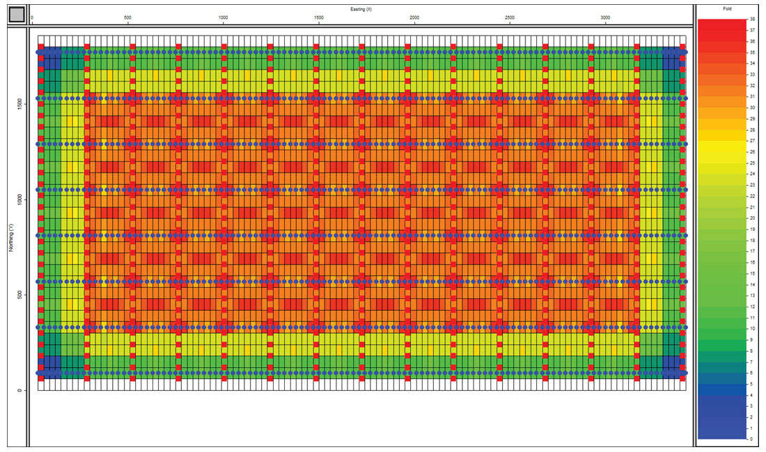
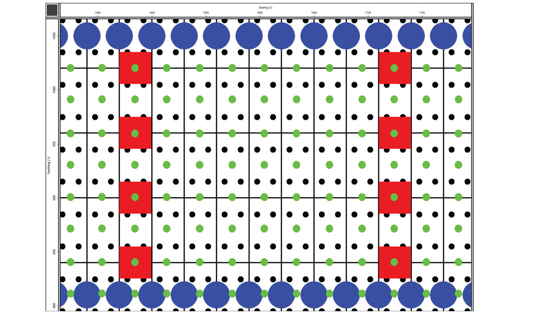
An orthogonal design employing the same design criteria (Table 1) is shown in Figure 2.
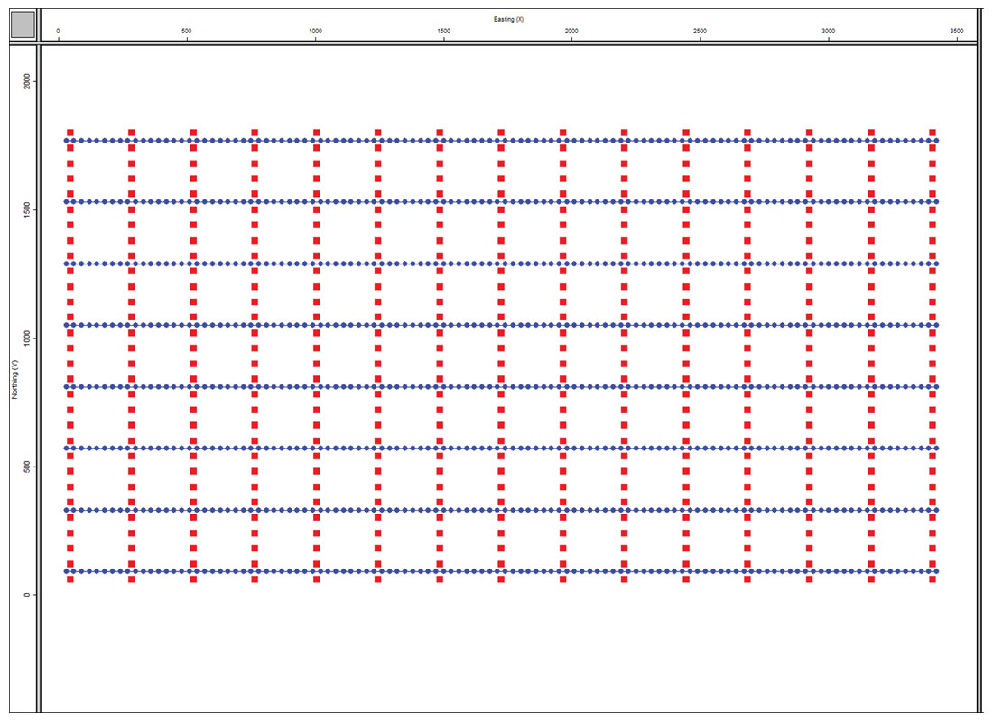
The set-up in Figure 2 is standard orthogonal cross-spread design. There have been no modifications using jitter, brick-work, diagonal, etc. Again field logistics would be favorable for an “all-live” patch. However, data with source to receiver offsets greater than 775 metres do not contribute to imaging the zone of interest. The operational statistics which determine the cost of acquisition are listed on the right side of Table 2.
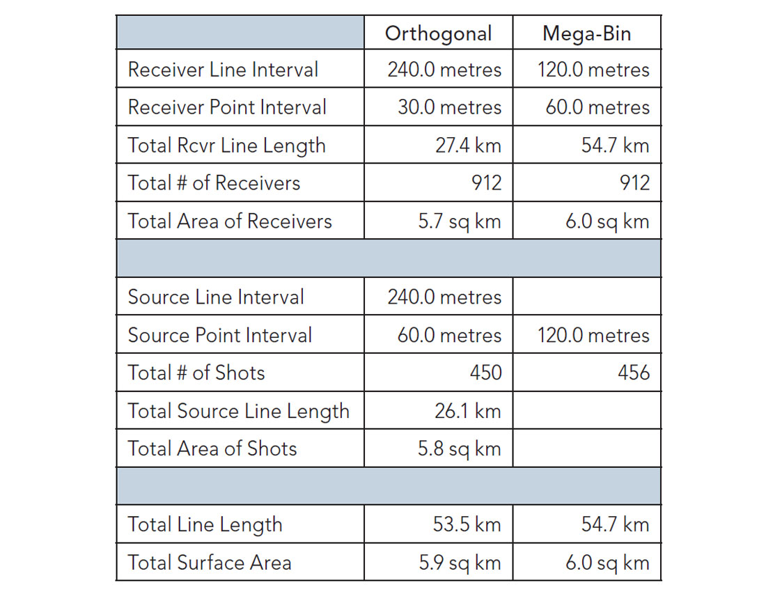
It is evident that both designs consisted of nearly the same number of shots and receivers. The land surface area occupied by each design was equivalent at 6 km2. And the total linear access length for sources/ receivers was the same at 54 km.
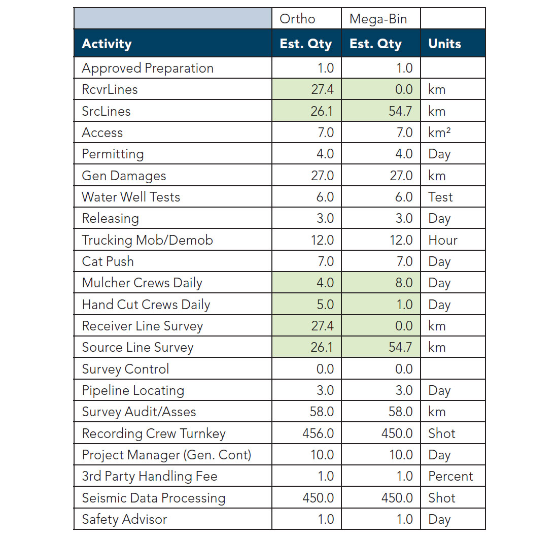
The cost drivers for acquiring each of these designs are identical. An example AFE is shown in Table 3. No matter what the costs are associated with the itemized project steps, the required resources are essentially the same, with the few differences highlighted. These small differences are due to the fact that for an orthogonal design the source and receiver line access are separate line items, but in the Mega-Bin design all line kilometres must be cleared for sources. For the orthogonal geometry, source and receiver line access are each about 27 linear km, whereas for the Mega-Bin all 54 linear km is source access. It might be noted that source line permitting and clearing is more expensive than receiver line permitting and clearing which results in a small cost uplift for Mega-Bin permitting and clearing. Each of the 2 survey types under consideration would incur the same cost to acquire within a very small margin.
Analysis
Each design is composed of the same number of receiver and sources distributed over the same areal extent. So the source and receiver densities are the same at 76 sources/km² and 154 receivers/km². Essentially all that was done was to rearrange the same number of sources and receivers into different patterns on the surface. The circular recording patch is the same for each survey.
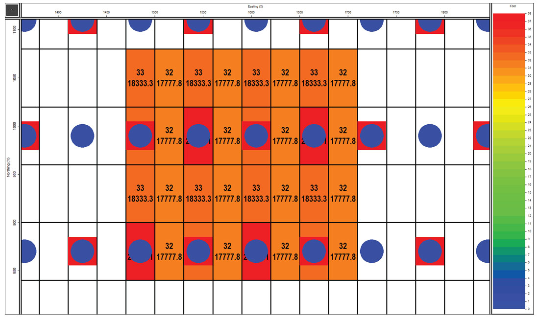
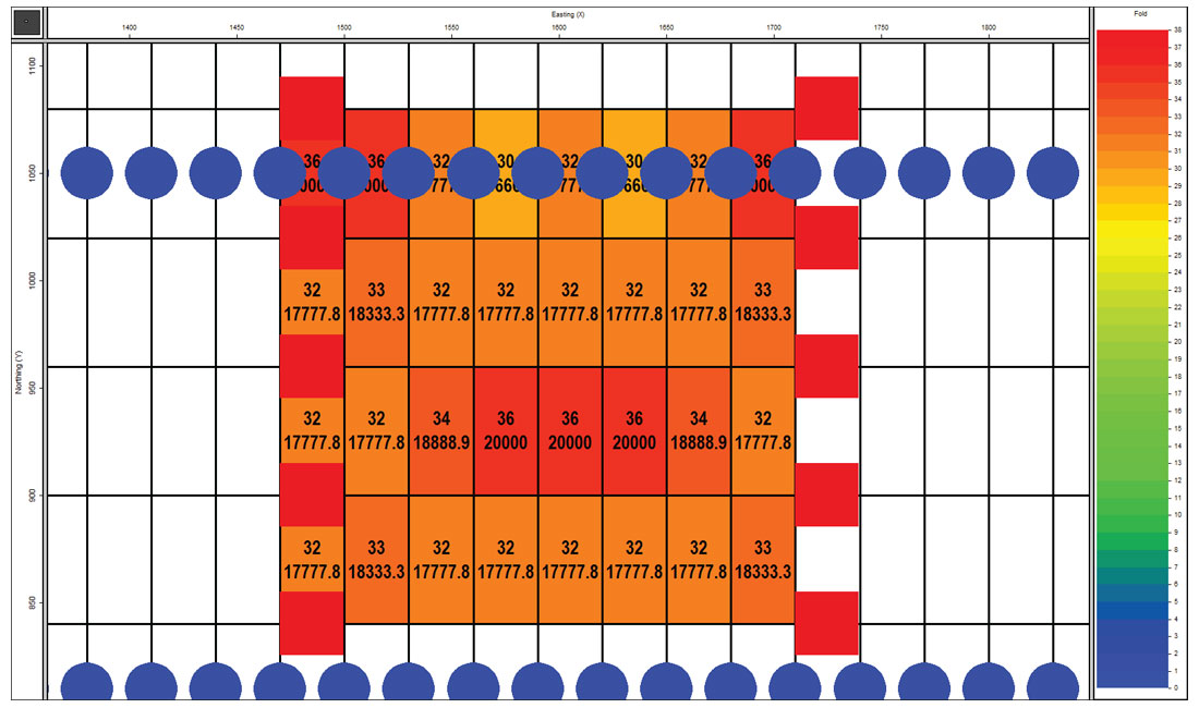
The natural subsurface bin size of the two surveys is different which can complicate the comparisons of trace density (Cooper 2004; Lansley 2004). To facilitate the trace density comparison both surveys are binned into 30 x 60 metre bins. In this manner the traditional CMP fold number correlates to trace density. Figures 3 & 4 are the subsurface multiplicity (fold) plots for each survey as binned into identical 30 x 60 metre bin grids and color coded with identical color bars.
It is clear that both surveys have the same full fold area of about 3 km². This can easily be calculated from the fact that full fold is achieved at about half the maximum offset distance, or at about 385 metres from the edges of each survey. Neither design has an advantage of a smaller surface area compared to full fold area. A close up view of the upper right corner is shown in Figure 5A and Figure 5B. The fold coverage builds up in different patterns, but full fold is achieved at the same distance from the edge of the surveys. The perimeter fold build-up area is the same.
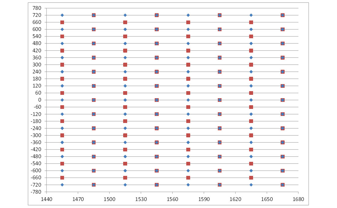
Within the full fold area it is beneficial to consider a repeating pattern of pre-stack traces when analyzing trace attributes. This insures that the analysis area has the same statistics as the full fold area as a whole. For the orthogonal survey design the pre-stack trace pattern repeats every 240 metres in each direction. For the Mega-Bin the pre-stack trace pattern repeats every 120 metres in the in-line direction and 240 metre in the cross-line direction. If two of the MegaBin repeating patterns are chosen and used to construct a 240 x 240 metre analysis area, then this new area also has the same trace statistics as a single 120 x 240 metre repeating area and the same trace statistics as the full fold area as a whole. However, now we can directly compare a 240 x 240 metre area from each survey in order to analyze differential statistics.
The 240 x 240 metre area chosen for analysis are shown in Figure 6A & 6B. In these figures the bins are color coded by CMP fold and annotated both in CMP fold and in trace density (traces/km²). In the Mega-Bin design the CMP fold varies from 32-38 (average = 33.1) [note the “38” annotation is hidden beneath a receiver symbol], which is a trace density of 17,777-21,111 traces/km² (average = 18,400). The orthogonal figure the CMP fold varies from 30-36 (average = 32.8), which is a trace density of 16,667-20,000 traces/km² (average = 18,200).
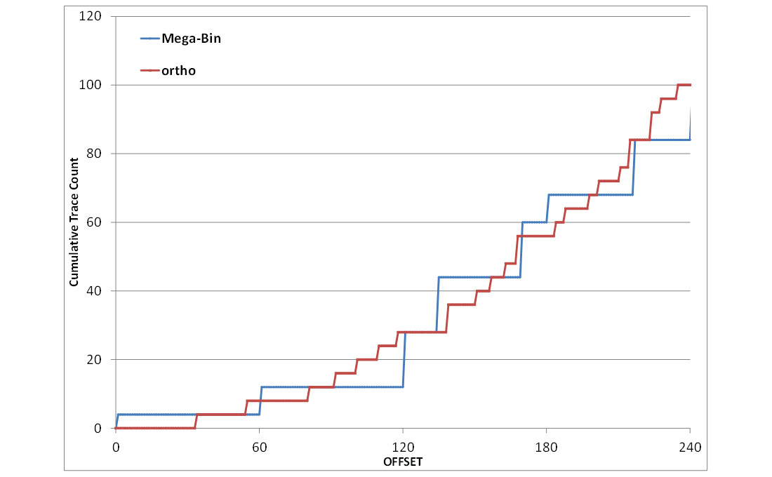
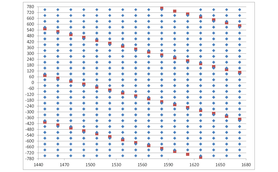
Within the repeating area the Mega-Bin survey contains 1060 traces and the orthogonal survey contains 1052 traces. When these traces within the repeating areas are plotted on a cumulative trace count versus offset it can be seen that the offset distributions of each survey are almost identical (Figure 7A). The traces for any given offset range are arranged differently within the repeating area, but their numbers are the same. Neither design has an advantage of higher trace counts in the near, mid, or far offsets.
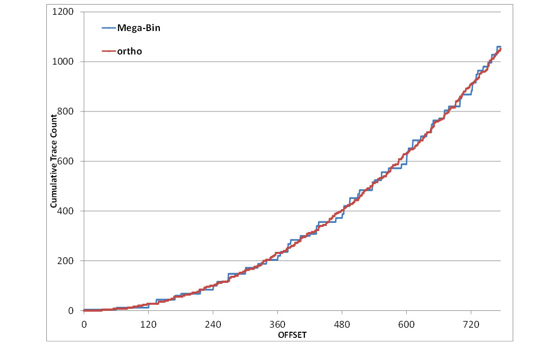
In Figure 7B the same data is plotted while zooming into the near 240 metres offset. It is still apparent that the two designs have the same population of very near offsets. The Mega-Bin repeating area contains four traces at zero offset. The orthogonal repeating area has four traces at 34 metres offset as the nearest traces.
The traces within the repeating areas can be plotted in a different way. In Figure 8A and 8B the traces are plotted according to inline offset versus crossline offset. This can be viewed as a lookup table of all possible trace offsets combinations within the survey. Every trace must be one of the points plotted in the figures. Moreover, within a repeating pattern there will be a contribution by every point in these figures. The Mega-Bin design consists of 265 unique combinations of inline/crossline offset (or radial offset/azimuth) in every 240 metre repeating pattern. The orthogonal design consists of 1052 unique combinations of inline/crossline offset (radial offset/ azimuth) in every 240 metre repeating pattern. The orthogonal design has 4 times as many unique inline/crossline (radial offset/azimuth) contributions than the Mega-Bin design.
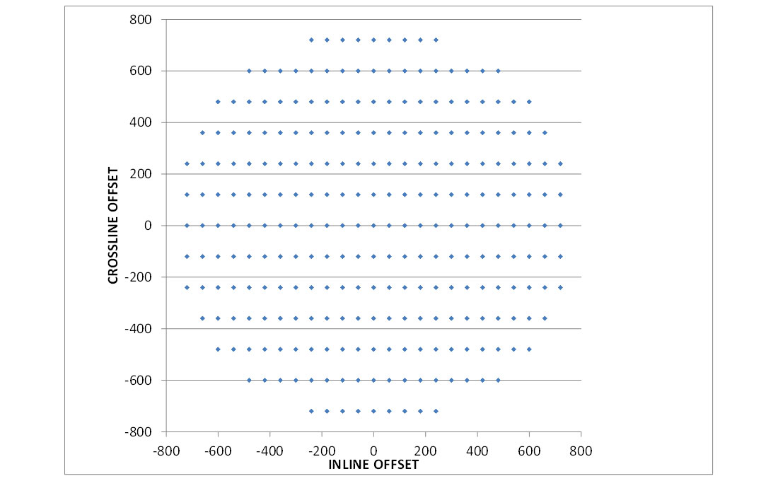
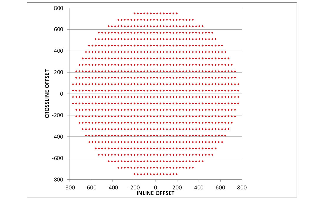
Inline offset and crossline offset are two of the four regularized dimensions in 5D regularization. Though the orthogonal design suffers more systematic variation in the inline/crossline (offset/azimuth) distribution, it should be noted that within a 240 x 240 metre area the orthogonal design will have 1052 unique locations in these dimensions available to the 5D interpolator. The Mega-Bin design will have 256 unique locations in these dimensions available to the 5D interpolator in the same 240 x 240 metre area. However, recall that we are using two of the Mega-Bin repeating patterns, so these 256 unique locations are in the inline/crossline dimensions repeat every 120 x 240 metres.
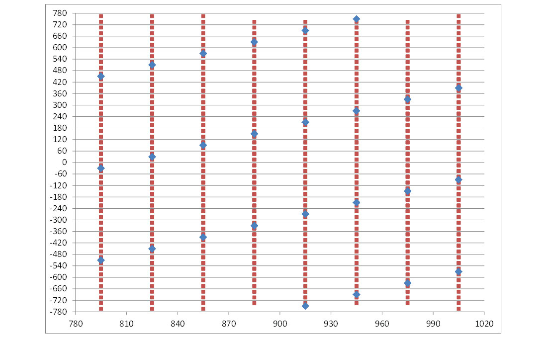
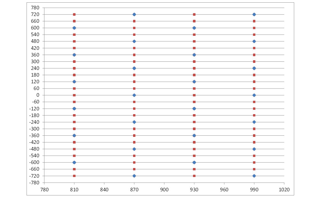
The other two dimensions in 5D regularization are midpoint-X and midpoint-Y. The Mega-bin design populates the X-Y space at a 30 x 60 metre regular grid. The orthogonal design populates the X-Y space at a regular 15 x 30 metre grid. The goal of the survey is to regularize the X-Y space to a 30 x 30 metre grid.
In Figure 9A the midpoint locations are plotted on midpoint-X and midpoint-Y axis [note some midpoints are hidden behind shot/receiver symbols]. Desired regularized locations (30 x 30 metre grid in the midpoint-X and midpoint-Y dimensions) are shown as green dots. If a black dot and green dot occupy the same location, the black dot overlays the green dot.
In Figure 9B the orthogonal design midpoints are plotted in plotted on midpoint-X and midpoint-Y axis as black dots. Also the desired regularized grid locations are shown as green dots. The orthogonal design is better populated in these two regularization dimensions.
Three of the four dimensions are visualized by plotting inline offset versus midpoint-X in one color and crossline offset versus midpoint-X in a different color, as shown in figures 10A and 10B. They show that within the repeating area for orthogonal design the crossline offset versus midpoint-X dimension is four times more densely populated than the Mega-Bin design. In inline offset versus midpoint-X dimension the Mega-Bin design is twice as densely populated as the orthogonal design and also uniform, whereas the orthogonal distribution is not uniform from this perspective.
Likewise plots using the fourth dimension, midpoint-Y, as the abscissa are shown in figures 11A and 11B. From this perspective the inline offset versus midpoint-Y dimension is four times more densely and uniformly populated than the Mega-Bin design. In crossline offset versus midpoint-Y dimension the Mega-Bin and orthogonal design have the same sample population. From this perspective the Mega-bin distribution is uniform, whereas the orthogonal distribution is not uniform.
The orthogonal design has more unique bin locations in all 4 dimensions. For 5D regularization to a 30 x 30 metre bin the input data from orthogonal design is oversampled in two of the four dimensions, midpoint-X and midpoint-Y. In the inline and crossline offset dimensions the orthogonal has a larger unique sample population The Mega-Bin design has a more uniform distribution from some, but not all, perspectives. Trad (2014) talks about aliasing in multiple dimensions and the complexity of quantifying the level of aliasing and, further, how aliasing is avoided by low temporal frequency filtering and carrying the low frequency localized information to the higher temporal frequencies. The finer sampling in the four regularized dimensions by the orthogonal survey design may allow a higher low temporal filter for reconstructing aliased portions of the wave field. An early demonstration of how finer and distributed sampling can facilitate beyond recovery was shown by Wisecup in 1998.
It is an avenue of further investigation to quantify the aliasing in 4 dimensions of each design. While this paper has looked at statistics within a repeating subsurface pattern it would also be useful to analyze Fresnel zone statistics. From that perspective the statistics will change spatially, temporally and by frequency.
Conclusion
The two survey designs considered both satisfy the minimum design criteria established by standard survey design analysis. They each have the same data acquisition effort and cost to image the same subsurface area and have the same trace densities.
Analysis of the pre-stack trace statistics shows that each have the same near, mid, and far trace offset population numbers.
The orthogonal survey design is more finely sampled in the four regularization dimensions which may lead to more effective 5D regularization or advantageous to other prestack multi-channel noise attenuation operating across these dimensions.

Acknowledgements
The authors would like to thank West Geophysical for support and ideas in developing this paper.


Join the Conversation
Interested in starting, or contributing to a conversation about an article or issue of the RECORDER? Join our CSEG LinkedIn Group.
Share This Article