Non-Hyperbolic Moveout, Polar Anisotropy and Anelasticity

Introduction

Experience with anisotropic velocity analysis shows that, occasionally, non-hyperbolic moveout in plains data cannot be satisfactorily corrected with the Grechka/Tsvankin approximation as presented at the 1997 SEG convention (Grechka and Tsvankin, 1997). For this approximation, a Taylor-series expansion is truncated beyond the fourth power in offset. In a subsequently published paper, Grechka and Tsvankin (1998) suggest a modification to their fourth power equation which can reduce the residual moveout. This modification is optimized below for minimum moveout error of a data example. In order to further improve on moveout correction errors, the Grechka/Tsvankin approximation is expanded beyond fourth order in offset for this study. However, even when anisotropic ray tracing is employed, which means there is no truncation of higher powers of offset at all, there persists a small and systematic moveout residual. As a further step, the assumption of anelasticity allows an additional reduction of the moveout correction error down to a level where the moveout residual is essentially random.

Polar anisotropy and non-hyperbolic moveout

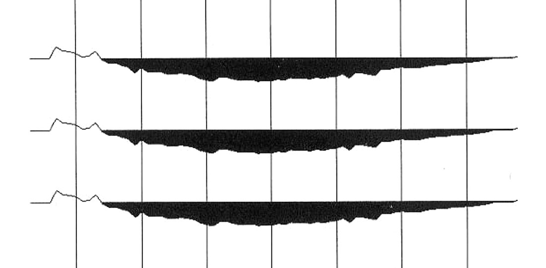
The specific real data example for non-hyperbolic moveout utilized in this study is shown in Fig. 1. This is a Dix-approximation NMO corrected common-offset display; two way travel time increases downward and offset increases to the left. Non-hyperbolic moveout is apparent around 500 ms, 640 ms and 860 ms. Residual moveout of the event at 642 ms is plotted in Fig. 2, again offset is increasing to the left. Residual moveout in this instance represents the difference between the actual data and the best-fit Dix-hyperbola. What makes Fig. 2 different from most other anisotropic velocity analysis cases is the presence of an inflection point. At small offsets the error curvature is convex upward and at offsets exceeding the inflection point the error curvature is changed to convex downward, creating some kind of bird-wing effect. This effect can be caused by shallow lateral velocity anomalies (Schneider, 1971), but no evidence for lateral velocity changes could be found in this case. Non-hyperbolic moveout can also be caused by drastic vertical velocity steps, even in isotropic settings (Harrison, 1989), or velocity gradients.

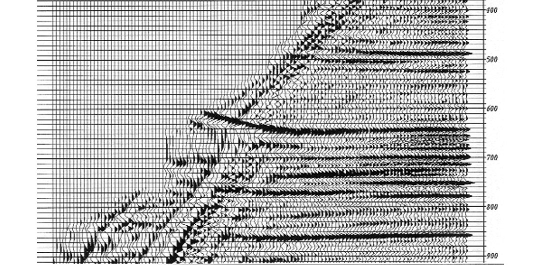
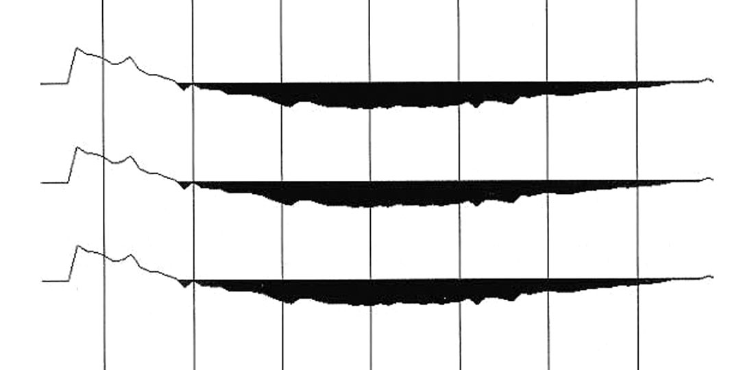
Fig. 3 shows the residual moveout resulting from isotropic elastic ray tracing; velocities are optimized for minimum moveout errors (minimum summed square errors). The difference between Figs. 2 and 3 is almost imperceptible; vertical velocity steps have very little influence on moveout characteristics in this instance. If vertical velocities change so smoothly with depth, maybe they should be modeled as a vertical velocity gradient altogether. The shallow part of a nearby well-log supports this idea. Fig. 4 is based on the assumption of a linear vertical velocity gradient, with the gradient computed for the same zero offset travel time and beginning velocity as was used for Figs. 2 and 3. Travel times in Fig. 4 are somewhat faster at large offsets when compared to the previous two displays because of a faster gradient end velocity, but the basic character of the moveout error curve has not changed and the inflection point is still present. Therefore it can be concluded from the above that the observed non-hyperbolic moveout is not caused by isotropic effects.

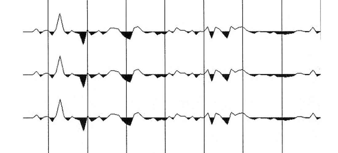
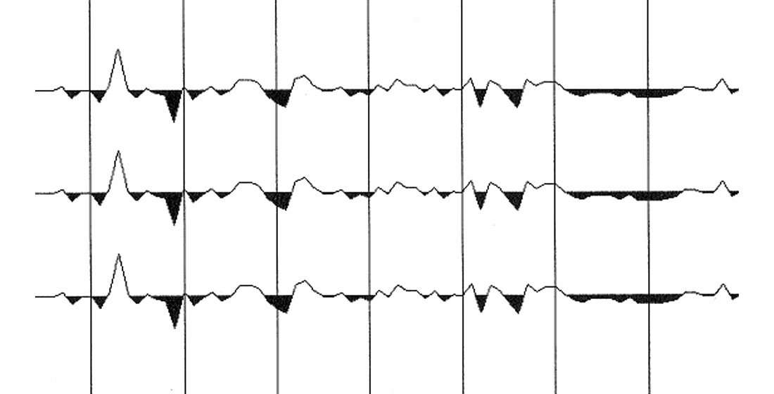
The Grechka/Tsvankin approximation to polar anisotropy (Grechka and Tsvankin, 1997) given in equation (1) is employed in computing the residual moveout shown in Fig. 5.

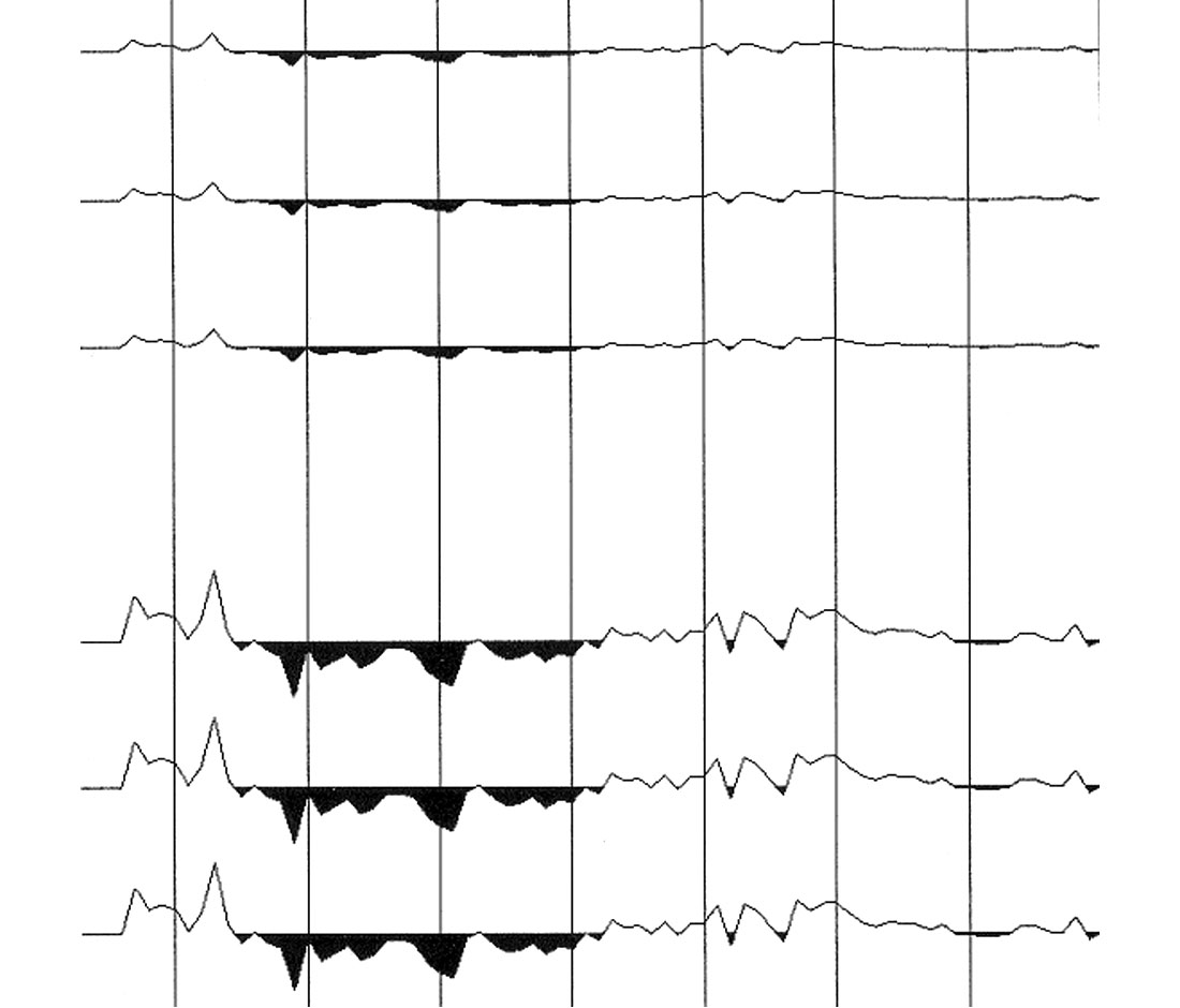
Horizontal and vertical velocities of this approximation are selected for minimum residual moveout, assuming a vertical axis of symmetry (VTI-type anisotropy). Equation (1) demonstrates the propagation direction dependence of anisotropic velocities. Vertical propagation at zero offset is controlled by the NMO-velocity. With increasing offsets and therefore increasing propagation angles (measured from the vertical axis) the horizontal velocity plays an increasing role. In the extreme of very large offsets, propagation is nearly horizontal and therefore is controlled mainly by horizontal velocities. Even though greatly improved when compared to the best-fit Dix-hyperbola result in Fig. 2, residual moveout is considerable and systematic in Fig. 5. The characteristic hockey-stick effect is clearly visible. The first group of three residual moveout curves in Fig. 5 is displayed at the same scale as Fig.2. The second group of three in Fig. 5 is a repeat of the first group, at four times the scale, in order to highlight the remaining residual moveout. Offset increases to the left, meaning at far offsets the moveout residual is positive, the actual data event travels faster than predicted by the approximation given in equation (1). A possible explanation for this moveout behaviour could be the fact that equation (1) is limited to fourth order in offset. Furthermore, because of the denominator of the term on the very right of equation (1), there is a roll-off to second order with increasing offsets. In order to more accurately describe the non-hyperbolic moveout at larger offsets in this specific case, offset terms beyond second order are required.

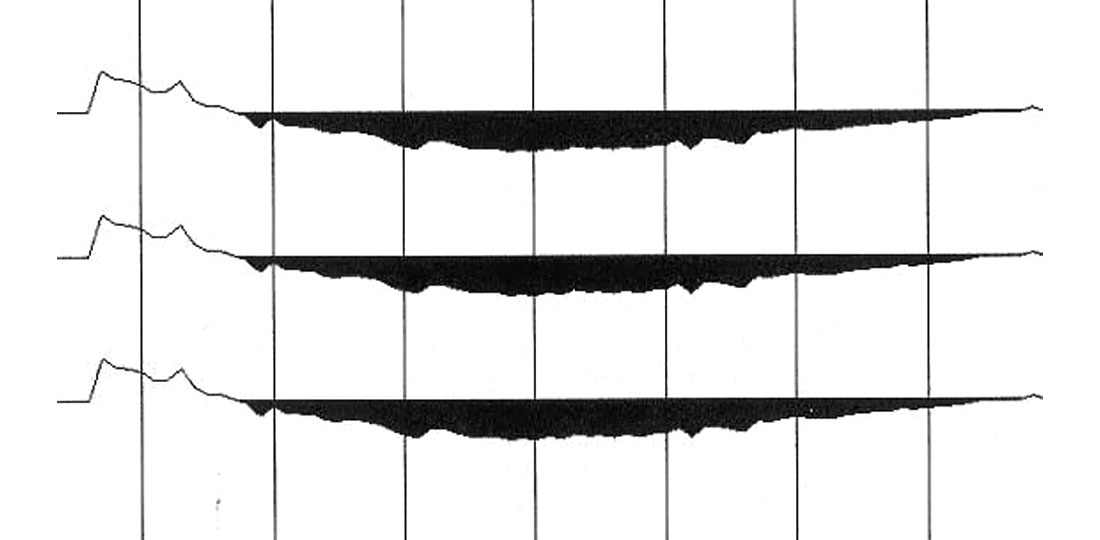
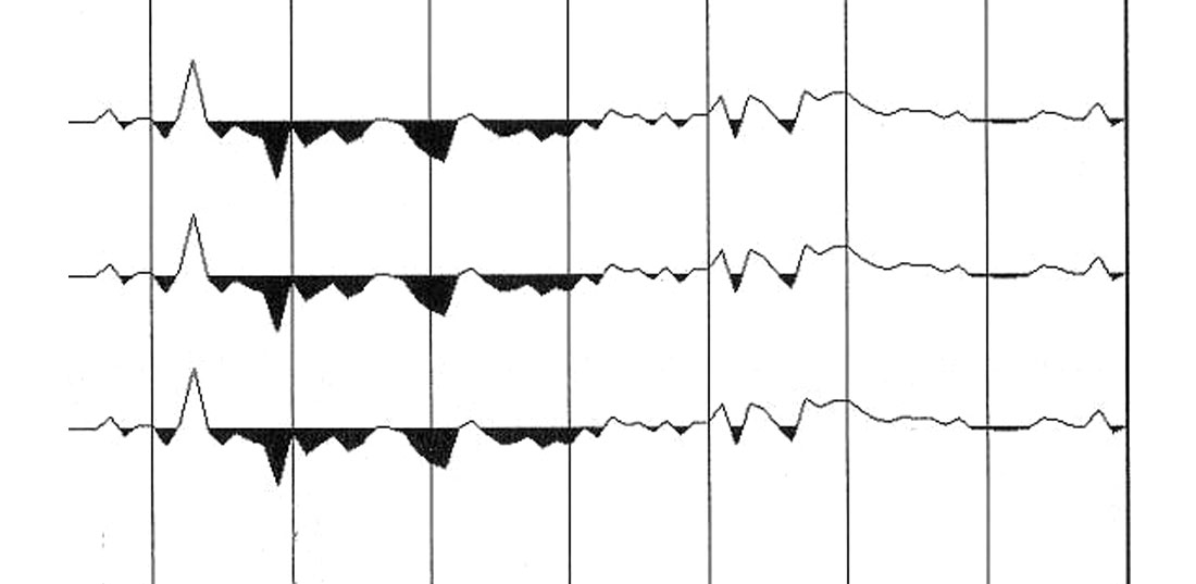
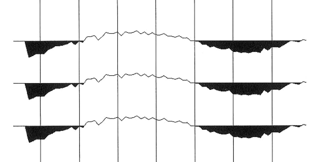
When anisotropic ray tracing is employed, no offset order restrictions are imposed. Fig. 6 shows residual moveout following anisotropic ray tracing, plotted at the same scale as the second (lower) part of Fig. 5. As expected, the hockey-stick effect has been corrected. Close inspection of Fig. 6 however reveals that a systematic moveout residual remains. Random noise in the data will cause a random moveout residual, but the systematic nature of the actually observed moveout residual (the bird-wing effect) suggests that the physics of the underlying processes leading to non-hyperbolic moveout are inadequately described. Thomsen parameters delta and epsilon (Thomsen, 1986) utilized in the anisotropic ray tracing leading to Fig. 6 are optimized for minimum residual moveout. Therefore, the systematic moveout residual cannot be explained by anisotropic effects.

Anelasticity and non-hyperbolic moveout

According to Aki and Richards (1980), the assumption of anelasticity leads to frequency dependent velocities and attenuation as demonstrated by equations (2) and (3).

Q in these equations is a frequency independent quality factor. Equation (3) gives amplitude decay per wavelength which is introduced by the definition of Q. Anelasticity is modeled here by invoking the linear theory of viscoelasticity (see also Krebes, 1980, Chapter 2), nonlinearities are not involved. As a consequence of equations (2) and (3), wavelet delay, wavelet amplitude attenuation as well as wavelet spread are observed, all increasing with travel distance; they increase more with lower quality factor Q. This is not surprising because higher frequencies are attenuated more with distance and as Q decreases, and the remaining lower frequencies travel at slower velocities. In other words, the frequency content of a wavelet is controlled by travel distance which in turn controls wavelet speed, leading to non-hyperbolic moveout.

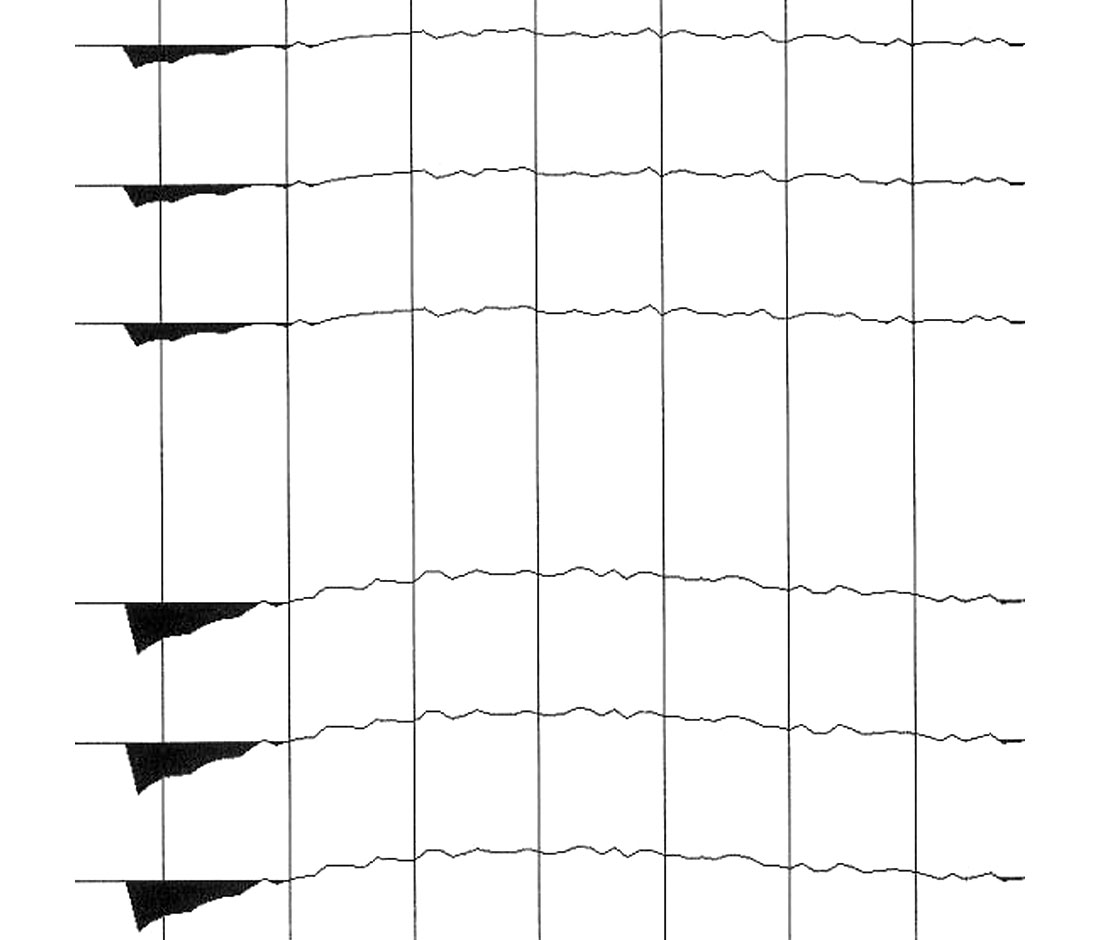
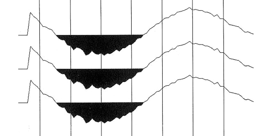
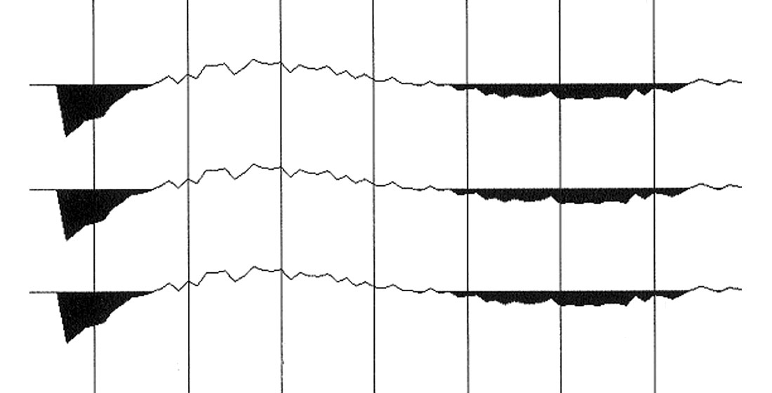
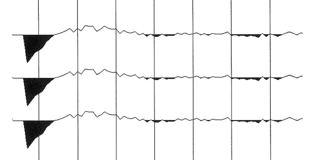
Fig. 7 is computed from a homogeneous, isotropic but anelastic model; offset is increasing to the left. The jitter is caused by numerical granularity of the anelastic moveout computation. Plotted are the moveout differences between model data and best-fit Dix-hyperbolae. The first group of three residual moveout curves in Fig. 7 is computed for Q = 50 and the second (lower) group for Q = 25, respectively. Not unexpectedly, the lower the value of Q is, the more non-hyperbolic the moveout curve. Fig. 7 shows that anelasticity causes far offset reflections to arrive later than the Dix approximation would predict, whereas polar anisotropy causes far offset reflections to arrive sooner, similar to Fig. 2. The moveout error curve in Fig. 7 is convex upward for all offsets. For weak and even moderate polar anisotropy, velocities are smoothly increasing with offset because of ever larger propagation angles to the vertical, thus giving a moveout error curve that is convex downward for all offsets. The residual moveout curve shown in Fig. 2 could be caused by a combination of polar anisotropy and anelasticity. In order to test this hypothesis, residual moveout of the data example in Fig.1 is now recomputed with anisotropic ray tracing and assuming finite Q-factors. Built into the polar anisotropic anelastic ray tracing algorithm is the assumption of Q-anisotropy as suggested by Waters (1987) and given in equation (4).

Thomsen parameters delta and epsilon as well as quality factors Q are optimized for minimum residual moveout. The result given in Fig. 8 is plotted at the same scale as Fig. 6. No systematic moveout residual as is observed in Fig. 6 can be seen in Fig. 8.

The non-hyperbolic moveout curve computed for the generation of Fig. 8 will be used as a basis of comparison for modifications to the Grechka/Tsvankin approximation described below. The moveout difference between the anelastic case in Fig. 8 and the elastic case in Fig. 6 is shown in Fig. 9, plotted at ten times the scale of Figs. 6 and 8. As in Fig. 7, the jitter in Fig. 9 is caused by numerical granularity of the anelastic moveout computation.

Fine tuning the Grechka/Tsvankin approximation

The factor of 1.2 in the denominator of the term on the very right of equation (1) was introduced empirically by Grechka and Tsvankin (1997) in order to minimize deviations from exact moveout in the offset range from 1.5 to 2.5 reflector depths. In a subsequent paper on non-hyperbolic moveout Grechka and Tsvankin (1998) re-iterate that, at intermediate offsets, their moveout approximation can be somewhat improved by empirically introducing a coefficient of C = 1.2, thus duplicating equation (1). The term controlled by factor C provides a roll-off to second order for very large offsets. As was observed before, the hockey-stick remnant in Fig.5 requires higher powers of offset for correction. Could equation (1) be improved upon in this specific case by shifting the roll-off to higher offset values? The residual moveout curve in Fig. 5 was obtained by picking horizontal and vertical velocities that minimize the sum of square errors. Can this minimum be further improved upon by including factor C as an optimization variable and thereby varying the roll-off point? An improved minimum is found indeed, at C = 0.62. Fig. 10 shows the residual moveout curve produced by C-optimization. The moveout difference between the anelastic optimum in Fig. 8 and the Grechka/Tsvankin optimum displayed in Fig. 10 is plotted in Fig. 11 at the same scale as Fig. 9. The Grechka/Tsvankin optimum in Fig. 10 is closer to the anelastic optimum in Fig. 8 than the elastic anisotropic ray traced optimum in Fig. 6 is, but a systematic moveout residual persists which is different in character from the elastic moveout residual.

The derivation of equation (1) is based on a three-term Taylor series approximation of non-hyperbolic moveout given by Hake et al. (1984). Expanding to a four-term Taylor series approximation and setting shear velocities to zero (as was done by Grechka and Tsvankin in deriving equation (1)) results in equation (5).

Optimizing equation (5) for minimum summed square moveout errors gives the moveout difference to the anelastic optimum (Fig. 8) plotted in Fig. 12 at the same scale as previous difference curves (Figs. 9 and 11). Fig. 12 shows a general decrease of moveout correction errors when compared to Fig. 11, but a somewhat weaker systematic moveout residual persists. There is also a curious error increase at the very largest offsets.

Comparing equations (1) and (5) leads one to speculate as to how to expand to the next power in offset beyond equation (5). Following this intuition (N.B. by speculation, not by arithmetic) leads to the optimization of three roll-off parameters C4, C6 and C8. A wide range of optimization starting points was investigated, but a thorough Monte Carlo search was not done; the moveout error minimum found might still not be the global minimum. This difficulty in dealing with increasing numbers of offset power terms is well known (see for example Al-Chalabi, 1973). Fig. 13 is the result of optimizing C4 to C8 and shows a further general decrease of moveout correction errors when compared to Fig. 12, with an increased error at the largest offsets. The systematic moveout residual has almost disappeared in Fig. 13.

The progression in the optimum data fit difference from Fig. 11 to Fig. 12 and to Fig. 13 appears to converge towards the anelastic optimum data fit. Stepping from equation (1) to equation (5) and beyond represents a more and more detailed polynomial fit of the moveout curve with an inherent parameter inflation. With ever increasing complexity of the polynomial even the noise in the data would be modelled, thereby ignoring the physics of the situation. The assumption of anelasticity by contrast introduces only one additional parameter, the quality factor Q in equations (2) and (3). Potentially, the expanded Grechka/Tsvankin equation (equation (5) and beyond) could camouflage anelasticity with anisotropy.

From the definition of Thomsen parameter delta (Thomsen, 1986) it is apparent that, for polar anisotropy, the moveout difference to the Dix approximation is convex downward at all offsets and delta is positive. The bird-wing effect present in the special data case considered in this study means the moveout difference to the Dix approximation is convex upward for small offsets and delta is negative. Indeed, as a result of “elastic” ray traced anisotropic optimization it was determined that delta/elastic = - 0.19 whereas “anelastic” ray traced anisotropic optimization gave delta/anelastic = + 0.01. This result immediately suggests a probing question. Table 1 in Thomsen’s classic paper (Thomsen, 1986) shows quite a number of materials with negative delta. Could some of those indicate hidden anelasticity?

Conclusions

For the specific real data example considered in this study, the best moveout correction is achieved by assuming anelasticity in addition to polar anisotropy.

Even though the bird-wing effect has been corrected by assuming anelasticity, this study is no proof that anelasticity is either the only or the predominant mechanism at work that explains the observed departure from anisotropic non-hyperbolic moveout. However, at the time of writing, anelasticity is the only mechanism known to the author to cause this kind of moveout behaviour in a 1D-earth. Whatever the cause for the observed moveout, simply approximating it by polar anisotropy must lead to errors in estimating velocities and Thomsen parameters.

A point completely ignored in the above investigation is the fact that deconvolution is applied in a normal seismic data processing run stream. Sudhir Jain (1986) states that anelasticity is compensated for by deconvolution. In the author’s experience deconvolution leads to over-compensation for anelasticity. The question of compensation or over-compensation appears to be connected to the size of the deconvolution operator design window. In the presence of anelasticity, wavelets change with depth and offset, which means the stationarity assumption is violated. The deconvolution process will modify non-hyperbolic moveout and also wavelet stretch. Optimum moveout correction is still possible, but velocities might be overestimated. This could explain why optimum migration velocities seem to be smaller than optimum stacking velocities in many cases.

In a recent paper on converted-wave reflection seismology, Leon Thomsen (1999) made use of a mathematical relationship similar to equation (1) in order to approximate non-hyperbolic converted-wave moveout. It is expected that the derivation leading to equation (5) for the pure-mode case can also improve approximations for the converted-mode case.

Acknowledgements

The author wishes to thank Talisman Energy INC. for the data example.