Introduction
Over recent decades, electromagnetic methods have been viewed with considerable suspicion by many in the hydrocarbon exploration industry. While highly effective in mineral and environmental geophysics, electromagnetic methods have played a minor role in hydrocarbon exploration. Since electromagnetic (EM) methods use signals that diffuse in the Earth, they cannot provide the same vertical resolution as modern seismic exploration. However, in the last decade, electromagnetic methods in general, and magnetotellurics (MT) specifically, have become more widely used in hydrocarbon exploration. This change is clearly not due to any change in the underlying physics but is due to:
- The significant improvements that have taken place in magnetotelluric data collection, processing and interpretation.
- The application of MT in settings where other exploration methods (seismic, gravity, magnetic) encounter problems, are cost prohibitive, or yield ambiguous results.
- The realization that MT data can provide complementary information to that derived from seismic exploration. For example, the diffusive signal propagation used in MT can be an advantage in a region of intense fracturing. While seismic signals will be scattered, the MT signals diffuse and give a reliable estimate of bulk properties such as porosity. Studies of the shallow structure of the San Andreas Fault illustrate the ability of MT to image rock volume properties (Unsworth et al., 2004).
Just as in seismic exploration, electromagnetic geophysics can contribute to effective hydrocarbon exploration in two distinct ways. Most often, EM methods are used to image structures that could host potential reservoirs and/or source rocks. In certain cases, they may also give evidence for direct indication of the presence of hydrocarbons.
In this article, the focus is on the magnetotelluric method as being representative of the developments in EM techniques in general. A review of the MT method is presented, recent developments are highlighted, and typical applications are discussed. Active source EM methods have seen a similar advance in technology and they have been applied to exploration for shallow gas and oil sand, or in a deep water setting. Table 1 summarizes the most common EM methods used in oil and gas exploration and outlines typical depths of investigation.
| Method | Source | Signal Type (Frequency Or time domain) |
Measured Fields (Electric or Magnetic) |
Depth of investigation in a sedimentary basin | Land or Marine |
|---|---|---|---|---|---|
| Table 1: Typical EM systems that have been applied to hydrocarbon exploration | |||||
| MT (Magnetotellurics) | Natural | Frequency | E and H | 1 – 10 km | Both |
| AMT (Audio-magnetotellurics) | Natural | Frequency | E and H | 100 – 1000 m | Land |
| CSAMT (Controlled sourc | Grounded Dipole | Frequency | E and H | 100 – 2000 m | Both |
| UTEM (University of Toronto EM) | Large Loop | Time | H | 50 – 500 m | Land |
| LOTEM/MTEM | Grounded Dipole | Time | E and H | 100 – 1000 m | Land |
| Land TEM | Loop | Time | H | 50 – 200 m | Airborne |
Basics of magnetotellurics
Magnetotellurics uses natural, low frequency electromagnetic (EM) waves to image the subsurface. These waves have frequencies in the band 1000-0.0001 Hz and originate in worldwide lightning activity and oscillations of the magnetosphere (Vozoff, 1991). These electromagnetic signals travel through the atmosphere as radio waves but diffuse into the Earth and attenuate rapidly with depth. The penetration depth is called the skin depth and surface measurement of electric and magnetic fields gives the average resistivity from the surface to a depth equivalent of the skin depth. The skin depth increases as frequency decreases, and thus a depth sounding of resistivity can be achieved by recording a range of frequencies as illustrated in Figure 1. At the highest frequencies (1000-300 Hz), the apparent resistivity equals the true resistivity, since only the uppermost layer is sampled. At intermediate frequencies, the apparent resistivity drops as EM signals penetrate the second layer. Finally, at the lowest frequencies, the resistive basement is detected.
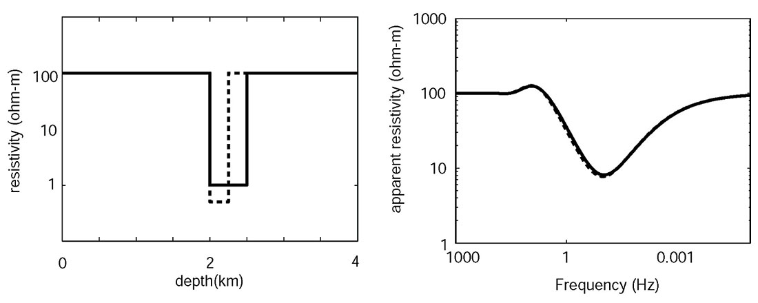
The best resolution is achieved in MT when determining the depth of a low resistivity layer, as in Figure 1, and this depth can generally be determined to within 10%. Unlike seismic reflection data, it is difficult to define formal resolution criteria. Another factor that must be considered is that MT is effective at defining the conductance (the product of thickness and electrical conductivity). However, the individual thickness and conductivity cannot be found, as illustrated by the second model shown in Figure 1.
The past
Through the 1970’s and 1980’s magnetotellurics was primarily used as a reconnaissance tool that could map variations in the thickness of major sedimentary basins (Vozoff, 1972; Orange, 1989). Data analysis was largely confined to 1-D forward modelling and inversion, an approach that could not be applied with confidence to areas of complex geology. Early efforts realized that MT was a potential tool for imaging conductive sedimentary rocks beneath thrust sheets of more resistive rocks such as carbonates, volcanics, and basement cored overthrusts (Anderson and Pelton, 1985; Berkman and Orange, 1985; Orange, 1989). In contrast to the small amount of MT work conducted in the west, hydrocarbon exploration in the former Soviet Union made more extensive use of all electromagnetic methods (see the review by Spies, 1983).
Modern magnetotellurics
The ability of modern MT to image subsurface structure has improved dramatically in recent years. This has been driven by developments in both instrumentation and interpretation.
Early MT systems were mounted in vehicles and required generators for power and an operator to be present for all data recording. This limited both access and the number of stations that could be collected per day by each field crew. These factors have been largely resolved with new MT systems, such as the Phoenix Geophysics V5-2000 and Metronix systems (see websites listed below). Modern MT systems are now very compact and generally fully automated. They can be carried by backpack to remote locations and left unattended to record time series data overnight. The dramatic reduction in equipment size is illustrated on the Phoenix Geophysics website listed below.
Another area in which major advances have been made is in the signal processing algorithms used to convert data from the time to frequency domain. Effective noise suppression through the remote reference technique requires synchronous recording at multiple stations (Gamble et al., 1979). In older MT systems this was usually achieved with very accurate clocks that were synchronized periodically. The problem of timing has been simplified with the use of timing signals from GPS satellites, provided the trees allow some view of the sky. Time series processing has benefited from the development of algorithms that use robust statistics to average the many estimates of apparent resistivity that are produced by a long time series. These methods effectively remove bad data segments in an automated fashion, resulting in a massive reduction in the effort associated with MT time series processing (Egbert, 1997; Larsen et al., 1996)
The advances listed above have allowed larger volumes of MT data to be collected and most interpretation is now made with 2- D and 3-D modelling and inversion algorithms. With a dense grid of stations, MT data can be fitted more closely since there is additional spatial redundancy in the data and model features are required by more than a single station. This allows data interpretation to proceed with greater confidence. Another major benefit from moving into 2-D and 3-D is that problems arising from static shifts and electric field distortion can be addressed. Static shift in MT data is similar to seismic statics and has the effect of introducing an unknown depth factor at each station (Jones, 1988). Many geophysicists who worked with MT data in the 1970’s were left with the impression that this was a fundamental limitation of the MT method. However, static shifts are now routinely removed in several ways. One approach is to independently measure the near surface resistivity with near-surface EM or DC resistivity surveys (Sternberg et al., 1988). An alternative approach is to allow the inversion algorithms to estimate the static shift coefficients and incorporate it in the model (deGroot- Hedlin, 1991). A debate continues regarding the various merits of these techniques and their philosophical legitimacy.
Overthrust exploration with MT
In many overthrust belts, major contrasts in velocity and/or resistivity can develop when different lithologies are placed above one another. If a high velocity thrust sheet is emplaced above lower velocity units, this contrast can present imaging problems for seismic reflection surveys. In addition, extreme topography and variations in weathering layer thickness in the overthrust terrain can cause large statics that make it impossible to acquire high quality seismic data. However, this geometry usually corresponds to high electrical resistivity over low resistivity, which is favourable for structural imaging with magnetotellurics. Christophersen (1991) describes a case study in Papau New Guinea that illustrates the effectiveness of MT in this context. A thick layer of clastic sedimentary rocks is located beneath 1-2 km of heavily karsted limestone. Seismic exploration in the region was complicated by statics and difficult access. In this type of survey, MT exploration requires a measurement site every 1-2 km, in contrast to the continuous profile needed for seismic reflection surveys. Watts and Pince (1998) describe a similar study in southeast Turkey, where near- surface structure again gives poor quality seismic data. In this study, the reservoir rocks were relatively resistive carbonates with sufficient resistivity contrast to be distinguished from the overlying assemblages of intercalated clastic sedimentary rocks and ophiolites. Dell’Aversana (2001) reports a study in the Appenines of Southern Italy and shows that low resistivity, underthrust sedimentary rocks are well imaged with a relatively broad station spacing (2-3 km). This study also shows that these data sets can benefit from a joint analysis of MT, gravity and seismic reflection data. The previous studies were able to derive useful structural information with just 2-D MT modelling and inversion. However, in some cases, more subtle contrasts can be masked by 3-D effects and a full 3- D analysis must be used (Ravaut et al, 2002). These case studies have shown that MT is an effective method of defining subsurface structure in overthrust belts and one contractor has reported collecting upwards of several hundreds of kilometers of profiles per year for these types of targets.
Seismic exploration in the Rocky Mountain Foothills has been very successful in defining detailed structure in many complex regions over the last 40 years. However, to date, significant use of electromagnetic methods has not been made. Early electrical and EM studies by Densmore (1970) showed that major resistivity contrasts were present, suggesting that structures could be imaged with electromagnetic data. Further tests of MT occurred in the early 1980’s in Montana and Southern Alberta but these projects were not followed up with more modern processing.
In 2002, the University of Alberta ran an MT profile in the Rocky Mountain Foothills to determine if useful structural information could be obtained in this geological setting. The profile began in the Alberta Basin and extended southwest from Rocky Mountain House, across the triangle zone and Brazeau Thrust Fault to the Front Ranges. MT data were collected using the University of Alberta Phoenix V5-2000 systems, supplemented by units loaned by Phoenix Geophysics in Toronto. MT data were recorded at stations located 2-3 km apart, typically placed at the roadside or in seismic cut lines. A recording interval of 18-24 hours per station was used and this gave estimates of apparent resistivity over the frequency band 100-0.001 Hz. MT data were simultaneously recorded at several locations to allow for noise cancellation through the remote reference method. Noise encountered in the survey came from cathodic protection on major gas lines and ground vibration from wind and traffic and was effectively suppressed with a combination of quiet recording at a remote station and robust time series processing algorithms.
The most important step in the subsequent processing is to convert the MT data from frequency to true depth. This is analogous to depth migration in seismic processing. In MT it is achieved through a combination of forward modelling and automated inversions in 2-D and 3-D (Rodi and Mackie, 2001). When these techniques were applied to the Foothills MT data, the model in Figure 2 was obtained.
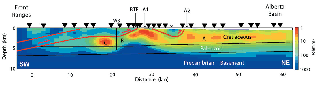
Interpretation of the resistivity model is possible using available well log information and comparison with coincident seismic data. The main features observed in the model are:
- A thick sequence of low resistivity units in the Alberta Basin (A). The pervasive low resistivities are primarily due to saline aquifers.
- The crystalline basement is resistive and dips gently to the southwest.
- A prominent low resistivity layer is located in the Cretaceous section. This unit rises in the triangle zone and is close to the surface northeast of the Brazeau Thrust Fault.
- Underthrust low resistivity units in the footwall of the Brazeau Thrust Fault, that can be traced a significant distance to the west (features B and C).
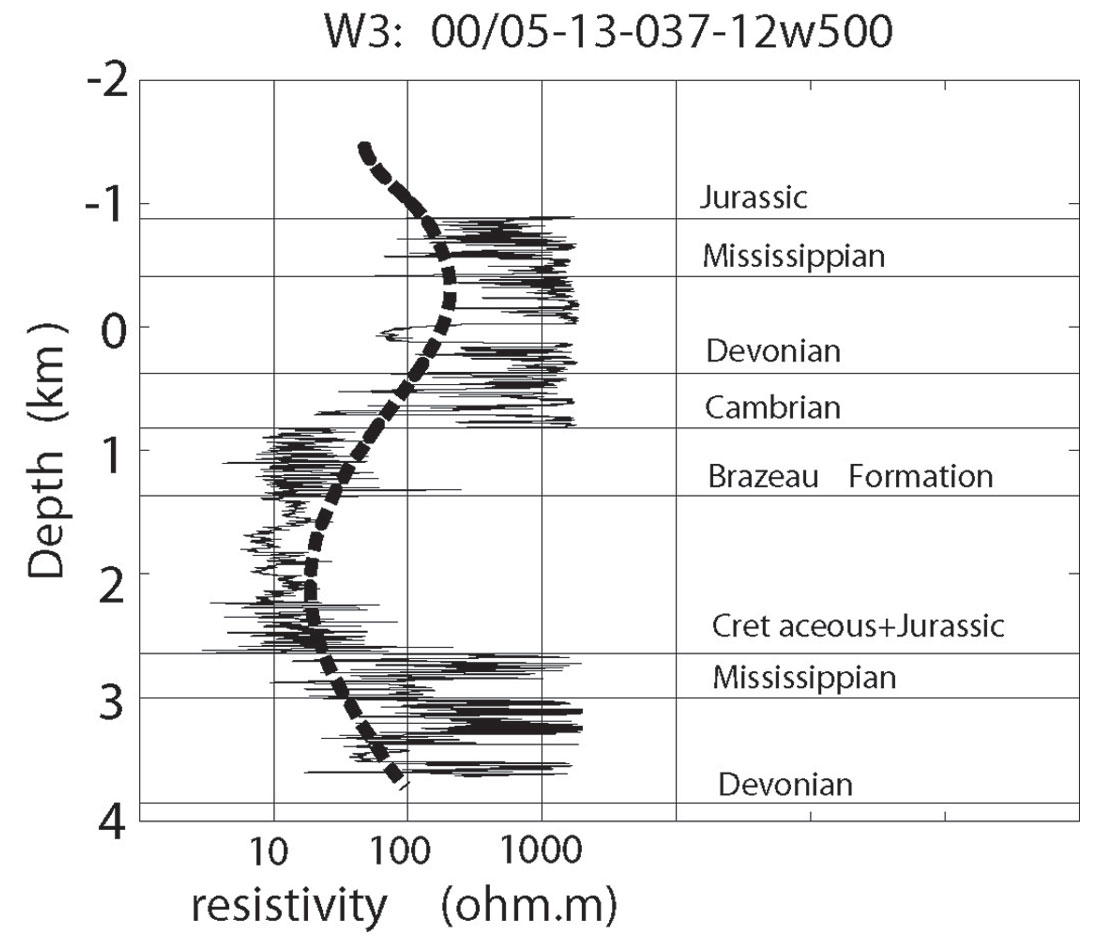
Figure 3, taken from Xiao and Unsworth (2004), shows the agreement between the MT derived resistivity and the resistivity log at a station southwest of the Brazeau Thrust fault. The MT resistivity model is spatially smooth, since it was derived with low frequency, diffusive electromagnetic signals with relatively long wavelengths. Note that the resistivity in the underthrust rocks is quite variable, with a pronounced zone of higher resistivities at 22 km (B) and lower resistivities at 18-20 km (C). These variations likely represent variations in the porosity of the underthrust sedimentary units, possibly related to a variable amount of fracturing. Archie’s Law can be used to estimate porosity from in situ resistivity and salinity data. Low resistivities are also observed in anticline A2 east of the Brazeau Thrust Fault and may delineate zones with fracture enhanced porosity.
Sub-basalt, sub-salt, and carbonate reef exploration
Determining the depth of sedimentary rocks beneath a cover of basalt is a similar problem to the overthrust case and success has been achieved with MT surveys. A number of studies were conducted in the Columbia Basin of Washington and Oregon (Prieto et al., 1985; Withers et al., 1994) and ongoing exploration in the area continues to use MT. Magnetotelluric exploration in the sub-basalt environment is also pursued in India (Deccan Traps), Russia (Siberian flood basalts) and Ireland (Tertiary Volcanic Province). Thick sequences of salt can mask seismic exploration efforts both onshore and offshore. Like basalt, salt is electrically resistive so EM methods are being used to image the base and sometimes the top of the salt. Examples from the Gulf of Mexico have been published by Hoversten et al. (2000). Tests of controlled source EM surveys for sub-salt imaging have been undertaken in the Colville Hills area of the NWT. Resistive pinnacle reefs in Southern Ontario have been mapped using several types of controlled source EM methods but the depth of investigation is small and resolution is poor (Phoenix Geophysics and University of Toronto).
Direct detection of hydrocarbons with MT
The results reviewed above have shown that MT can image structures that could host potential hydrocarbon reservoirs. The study in the Foothills has shown that it may also allow variations in porosity and pore fluid salinity to be mapped. Can MT directly image the hydrocarbon reservoirs? Outside of the Russian literature, there are very few published studies that definitively show success in this area. The most common problem encountered by MT is the possible masking of a response from an oil/gas saturated reservoir by changes in lithology. Another factor that reduces resolution is that the electric currents used in MT flow in an essentially horizontal direction. Thus horizontal, high resistivity layers are essentially invisible since they have little effect on the horizontal electric currents. However, controlled source EM methods generate electric currents that flow in both the horizontal and vertical directions and have better resolution to allow direct detection of hydrocarbons. Case studies include the seafloor examples listed below and apparent changes in subsurface resistivity over time as gas was added and removed from a shallow reservoir (Ziolkowski et al., 2002).
Marine magnetotellurics and controlled source EM methods
The last decade has also seen the rapid development of EM methods that are useful for hydrocarbon exploration in the marine environment. Marine magnetotellurics was developed in the 1980’s and initially applied to studies of the lithosphere and mid-ocean ridges (Evans et al., 1999). The seawater in deep oceans, a major conductor, screens out the high frequency signals (above 0.01 Hz) needed to image structure in the upper few kilometers of the seafloor. However, with modern recording equipment in low noise environments, higher frequency signals can be detected in moderate water depths (Constable et al., 1998). Controlled source EM methods were also initially developed for mid-ocean ridge exploration (Unsworth, 1994) and have subsequently been applied to shallow hydrocarbon exploration. These methods use a ship to tow a transmitter over an array of seafloor instruments providing coverage of an exploration area (Eidesmo et al., 2002). The presence of the conductive seawater reduces natural noise and allows weak signals from the subsurface to be detected. A combination of low resolution MT and higher resolution controlled source EM is becoming the preferred method for mapping the background sedimentary section and detecting discrete resistive layers. The recent development in this field builds on decades of university, government and commercial research on seafloor electromagnetics involving groups in Canada, USA, UK, Japan, Australia and France.
The future
Despite the limitations of MT in the early days of its application to hydrocarbon exploration, the method has matured into a tool that works effectively in certain niche environments. Since the limitations were understood, it has proved to be a valuable complement to other exploration methods. Today large amounts of MT data can be collected rapidly and cost effectively to provide the density of measurements required to image complex geology. The next innovation in EM may come from data processing, interpretation and the integration of surface and borehole methods to improve vertical resolution.

Acknowledgements
MT data collection in the Rocky Mountain Foothills was funded by research grants to Martyn Unsworth from NSERC, the Canadian Foundation for Innovation, Alberta Ingenuity Fund, ISRIP and the University of Alberta. Fieldwork was also supported through technical help and equipment loan from Phoenix Geophysics. Discussions with Don Watts and Richard Kellett over recent years are gratefully acknowledged.


Join the Conversation
Interested in starting, or contributing to a conversation about an article or issue of the RECORDER? Join our CSEG LinkedIn Group.
Share This Article