Natural fracture characterization from 3D structural attributes

As seismic interpretation continuously evolves, it seems that interpreters have not kept pace with technological innovation provided in commercial software: workflows may be more persistent than technologies. Despite having access to 3D seismic for close to three decades, the majority of an interpreter’s time is spent picking inline and crosslines profiles with the objective of making surfaces.

The aim of this paper is to make a snapshot of the current seismic interpretation practices commonly used, and to provide a possible alternative workflow that will allow geoscientists to spend their valuable time on interpreting the sub-surface rather than picking seismic. This workflow automates most of the otherwise tedious picking of the structural and stratigraphic information, and then converts the seismic and interpretation data into the chrono-stratigraphic domain, representing the theoretical time of deposition of the sediments. A useful application of this workflow is the prediction of fracture probabilities given geomechanical rock properties.

Geophysical interpretation history

Seismic data, and well log data, are used to develop an understanding of the earth’s interior. Such an understanding is generically termed a ‘model’ of the earth, or an ‘earth model’. Prior to the widespread use of computer workstations the geoscientist’s earth model was purely a 2D construction: plan view maps constructed from 2D profiles in the case of seismically derived ‘models’, and plan view maps and 2D cross sections derived from point data in the case of geologically derived models. 3D renditions of the model lived inside the heads of the geoscientists themselves; difficult to share amongst an asset team in the manner that a modern geo-cellular software model is shared.

Approaching three decades after the introduction and subsequent rapid improvement of 3D seismic data and workstation software the workflows remain largely two dimensional: correlate seismic data to logs; pick major reflectors on generally orthogonal sets of 2D profiles, generate surfaces. Then iterate with increasing attention to subtlety to reveal and map smaller features. Somewhere in the procedure time/depth conversion is undertaken. It is a legacy workflow familiar to geophysicists who started their careers working on 7.5 inch / second paper plots using a yellow pencil and a timing ruler – including one of the co-authors of this article. Workflows persist in part because the industry relies on experienced practitioners to mentor new graduates. The most influential period in any ‘journey’ is the beginning – the formative workflows learned in one’s early career are passed on across generations. While valuable and appropriate, this dynamic may fail to exploit the power of modern software, and may fail to position all workers to be effective in the face of rapid change.

The legacy workflow emphasizes the production of surfaces. Time structure surfaces are generated and used to build depth structure surfaces and isochron/isopach grids. Effort, time and ‘mindshare’ are typically focused on the generation of large surfaces – ones that are consistently mappable over large areas of the seismic survey area. Mapping the richness of geometrical and geomorphological information contained in aerially smaller reflections or reflection fragments tends to take a lower priority due to the time involved in more or less manually picking over the survey area. While effective for conventional hydrocarbon extraction projects, the legacy workflow may fall short when viewed in the context of the increasing demand for understanding heterogeneity imposed by so called ‘resource’ hydrocarbon extraction projects (typically scalable, repeatable, tight, impermeable and/or self-sourced).

An alternative workflow is proposed wherein automated reflection horizon tracking is used to pick a very large population of reflections, including reflections limited in area which we call stratigraphic trends. The geoscience team (geophysicist, geologist, geomorphologist) are able to spend more time, after appropriate quality check, interpreting the results; by which we mean they spend time extracting geological insight from the seismic data and the suite of ‘trends’ and capturing that insight in geological modeling software.

Automating the geophysical interpretation workflow

There are many workflows available to the interpreter to extract valuable subsurface insights. Geoscientists should take advantage of what can be automated (without compromising for interpretation quality) to allow time to be spent on what matters.

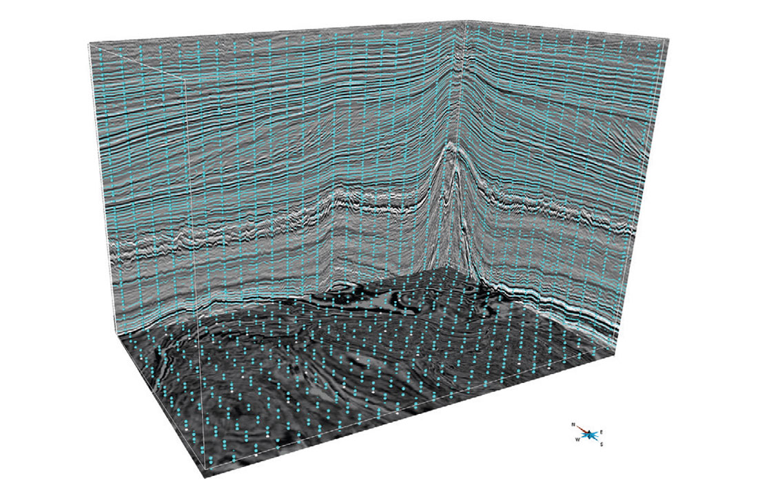
Starting from a seismic line or volume, thousands of seismic reflector patches can be automatically picked. Thousands of seeds are dropped at a user specified bin spacing and then snapped onto seismic reflectors (peaks, troughs or zero-crossings). Each seed point is then being used to auto-track patches following a seismic reflector. The workflow then automatically discards the patches that are too small to be relevant and merges the overlapping patches (Figure 1).

Automating the picking of seismic frees the geoscientist’s time for real interpretation: checking the validity of the trends extracted and making sense of them geologically. Working with thousands of trends means a lot of data to check. To quickly scan through them, the geoscientist can sort the trends by various attributes (size, location, chrono-stratigraphic age, dip, azimuth…).

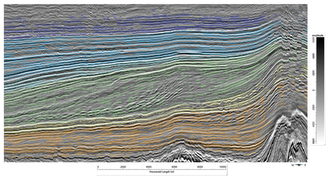
A typical workflow usually starts with a first pass using sparse seed points to extract the main continuous events that can be interpreted as key seismic stratigraphic horizons. Then a second pass within each stratigraphic unit with a much higher density of seed points will extract most of the relevant stratigraphic trends (Figure 2).

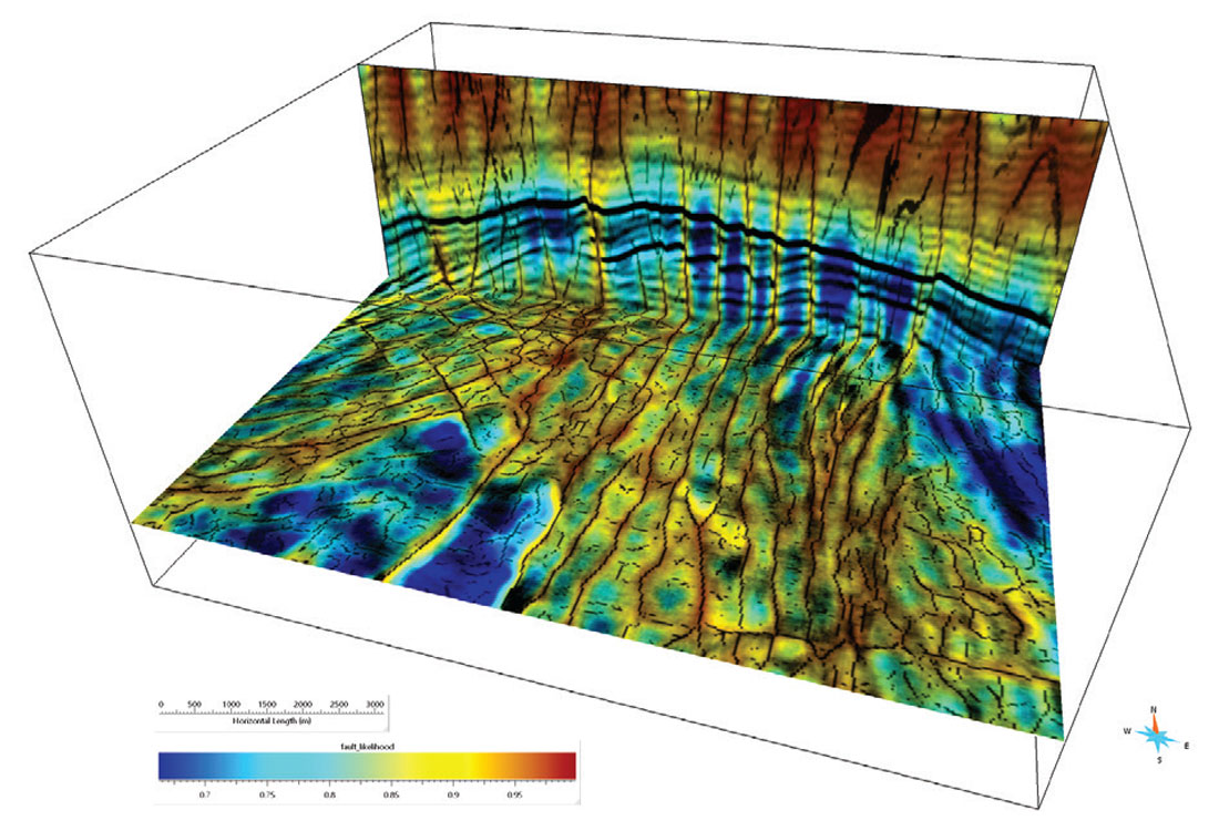
Another part of the interpretation workflow is to extract faults. They can be interpreted using fault attributes of likelihood, strike and dip. The method used to compute these attributes is based on semblance (Taner and Koehler, 1969), and is therefore similar to methods proposed by Marfurt et al. (1998). Like Marfurt et al. (1999), semblances are computed from small numbers (3 in 2D, 9 in 3D) of adjacent seismic traces, after aligning those traces so that any coherent events are horizontal. The fault likelihood attribute is then scanned over multiple fault orientations in order to find the strike and dip angles that maximize the fault likelihood. When complete, the results of this scan are images of maximum fault likelihoods and corresponding fault strikes and dips (Hale, 2012) (Figure 3).

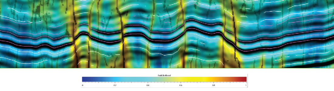
Faults surfaces can then be picked automatically or manually using the maximum fault likelihoods. A good way of identifying the faults surfaces to interpret is to display the seismic amplitude (gray scale), co-rendered with the fault likelihood attribute (bright color scale) and the thin fault-likelihood attribute (black intensity), with the stratigraphic trends (Figure 4). The trend terminations often line up with the high fault likelihood and therefore help the interpretation of fault surfaces.

A particular advantage to a workflow involving semi-automatic extraction of faults, horizons and stratigraphic trends is that geoscientists are letting the data talk, while spending their valuable time checking the quality and validity of the automatically interpreted data.

But geoscientists should not stop at the interpretation of the faults, horizons and stratigraphic trends. Historical boundaries between interpretation and modeling are being erased with the implementation of full seismic interpretation tool kits within most major commercial geomodeling software. This offers the opportunity to model while interpreting. The challenge for geoscientists is to learn how to take advantage of this: traditionally, interpreters are not modelers, and modelers are not interpreters.

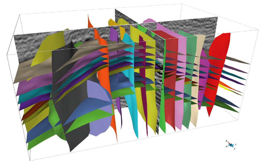
Fortunately the construction of 3D structural models has also been simplified. All the faults, horizons and stratigraphic trends extracted can be used to automatically build a fully sealed 3D structural model where the horizons are interpolated using geological rules that honor the stratigraphic column and associated layering structure, and are properly truncated against fault, salt, and erosion surfaces (Figure 5). This is done using the concept of space/time mathematical framework introduced by Mallet (2004, 2008). In this framework, the subsurface is curvilinearly parameterized by a uvt-transform which maps every (x,y,z) point in the geological space to a (u,v,t) point in the parametric space. The uvt-transform is computed such that an iso-t surface corresponds to a stratigraphic horizon and an iso-t is discontinuous across the faults (Labrunye et al., 2013).

A huge advantage for the interpreter is that the process automatically creates a full 3D chrono-stratigraphic time volume, where the data has been restored to the time of deposition. This means that the seismic volume is unfolded and unfaulted.

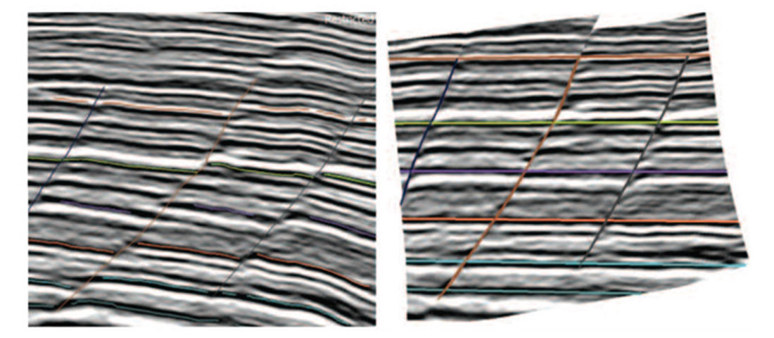
There are many applications to working in the chrono-stratigraphic domain. The first one is the ability to easily and quickly validate (and correct if necessary) the structural and stratigraphic interpretation. If all the faults and stratigraphic events have been picked correctly, then all the reflectors should be flat and no fault throw should be visible on the seismic in the chrono-stratigraphic domain (Figure 6).

The chrono-stratigraphic domain is also useful to facilitate the interpretation of geomorphologic features as discussed by Dulac (2011), Labrunye et al. (2013) and Thenin et al (2013). Another novel application of the conversion of a seismic volume to the chrono-stratigraphic domain is the estimation of fracture probability.

Application to shale and tight reservoirs exploration

Most geophysical studies in unconventional gas rely on inversion techniques and simple structural attributes to characterize the natural fractures of reservoirs. These studies tend to overlook the structural and stratigraphic information embedded in 2D and 3D seismic data and do not typically use geomechanical data as input.

The 3D structural model derived from the seismic interpretation can be converted into a 3D geological grid without loss of structural or stratigraphic information. The geological grid represents the final state of deformation that took place between the time of deposition of the horizons (chrono-stratigraphic domain) and today (geological space). A one step structural restoration to the state of deposition, before all the deformations, is done assuming the horizons are deposited horizontally and given the location of each part of the geological grid truncated by the faults.

The dilatation is computed on the geologic grid using the uvt-transform previously defined and the geomechanical parameters of the rock. The dilatation takes into account the sum of deformations from the time of deposition (state without deformation) to now (state which has registered all the deformations of the field). It is computed as (Volume of the actual time – Volume at time of deposition) / (Volume at time of deposition). This gives local information on the type of deformation the structure has undergone (compression where dilatation is negative and extension where dilation is positive) with the sum of deformations of the field (Prieto-Ubaldo et al., 2014).

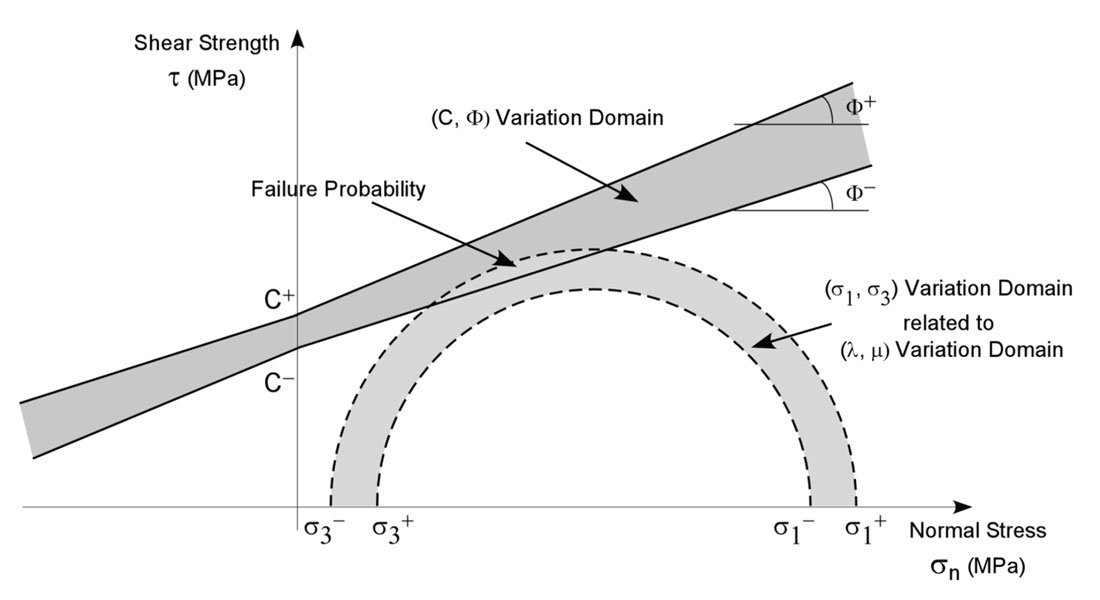
The uvt-transform links both the geological grid at time of deposition (chrono-stratigraphic domain) and the geological grid at present state (geological space) which has undergone the sum of all deformations which have affected the field. The vector of displacement for each grid cell between the moment of deposition and present is consequently known and allows the computation of a strain tensor. The stress tensor is computed from the strain tensor using Hooke’s law and the Lame’s parameters (computed from the Poisson ratio and the Young modulus). The sensitivity of the rock material to the fractures can be assessed through a failure criterion, like the Mohr-Coulomb criterion (using Mohr-Coulomb cohesion and friction angle parameters). Ranges of geomechanical parameters values are used in order to take into account their uncertainties, allowing the computation of a fracture probability (Mace, 2004) (Figure 7). The fracture probability estimation is assuming that the natural fractures present in the reservoir have been created by the deformation which produced the faults and folds (structural deformation) of the study area.

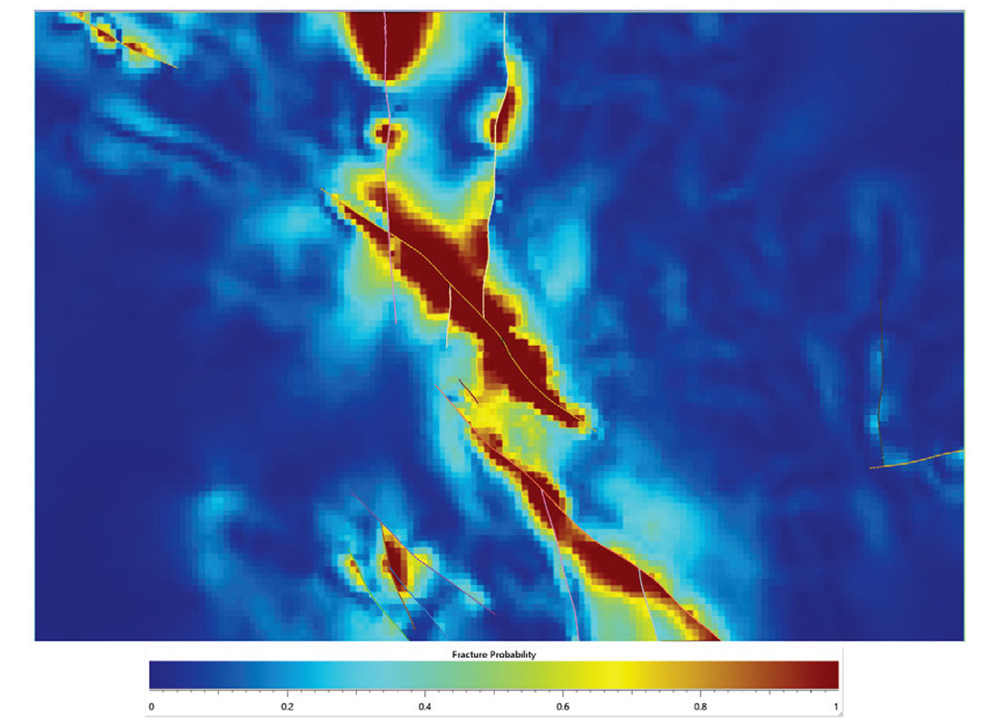
This fracture characterization workflow has been applied as a sweet spotting technique in prospective shale formations in Northeast BC, Canada (Figure 8).

The fault and fracture attributes prediction should then be cross-validated at the wells with the available natural fracture information (from core description and FMI interpretation), the initial production volumes and the fracking related information (stimulation interval, volume of injection, microseismic).

Conclusions

Automating the seismic interpretation and coupling it with the 3D structural modeling workflow enables geoscientists to extract as much structural and stratigraphic information as possible from seismic amplitude data and to work in the chrono-stratigraphic domain.

In addition to being useful to validate the interpretation, the chrono-stratigraphic domain provides new applications to geoscientists to help better characterize the sub-surface. An important one is the ability to characterize natural fractures stratigraphically. This has proven a valuable sweet spotting tool for shale gas exploration in Northeast BC. This natural fracture characterization workflow provides several advantages compared with traditional seismic characterization workflows. It helps reducing project cycle time by automating the otherwise tedious interpretation of faults and horizons from seismic and it does not rely on pre-stack inversion.

Acknowledgements

The authors would like to thank Stanislas Jayr and Emmanuel Labrunye for the many technical discussions on the subject of seismic interpretation and modeling over the years, as well as Tony Wain and Thomas Jerome for their comments and feedback.

The authors would also like to thank F.C. Marechal, Quicksilver Resources Canada Ltd., for permission to show pictures to illustrate this paper.

The authors would also like to thank dGB Earth Sciences B.V. and TNO for making the Netherlands Offshore F3 Block 3D survey dataset available through the Open Seismic Repository.