Modelling and imaging of an impact structure

Introduction

Of the more than 150 impact craters currently known, approximately 25% are associated with economic deposits and 17 are being actively exploited (Grieve and Masaytis, 1994). Brown (2002) highlighted the two most interesting aspects about the petroleum potential of impact craters: 1) mixed breccia deposits that formed during the impact make excellent reservoirs; 2) more than one part of the impact structure can host hydrocarbon accumulations. Mazur and Stewart (1997) provide an excellent review of impact structures currently investigated by CREWES, the Applied Geophysics group at the University of Calgary. In addition to its significance for the scientific community, crater research is aimed at extending the current knowledge about the hydrocarbon potential of impact structures.

Kirtland Grech et al. (1998) carried out a modelling experiment of a thrust model with a complex velocity structure, and compared a number of pre-stack and post-stack migrations. The authors discussed the performance of each method in positioning and focussing a number of reflections that are typical of thrust environments. More recently, Isaac and Lines (2002) compared pre-stack depth migration to pre-stack time migration. They created synthetic seismic data by ray-tracing a depth model with vertical and lateral velocity variations and showed that time migration in some cases does not position events accurately, even when the exact velocity field is used for migration.

In a similar way, I created an original geologic model of a complex impact crater, ray-traced the model, then pre- and post-stack migrated the resultant seismic data in depth and time using Kirchhoff migration. The objective of the study was to to compare the results and merits of the various methods, and to determine which events are better imaged and which are less well imaged, if any.

Geological Model

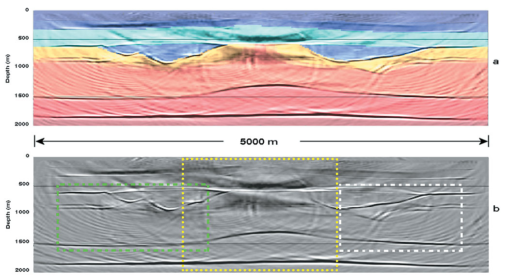
Figure 1 (Westbroek and Stewart, 1995) summarizes the features of interest in a complex crater, including normal faults and slumped blocks in the rim, breccia deposits and a well-developed central peak with upturned layers. Figure 2 is an example interpreted seismic section across the Hotchkiss structure (Mazur et al., 1999).

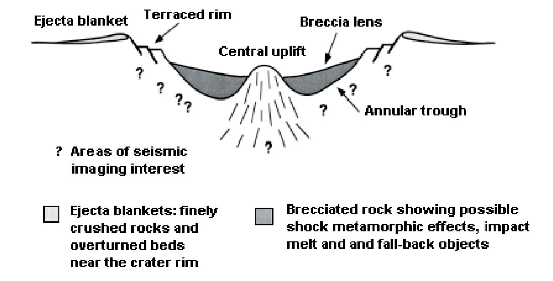
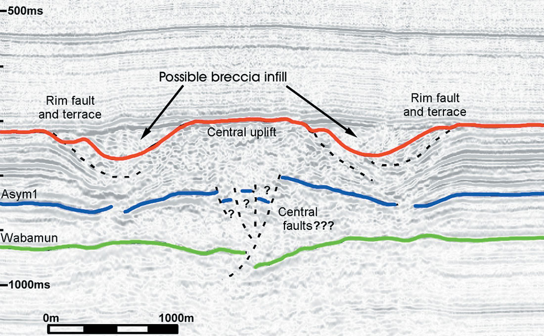
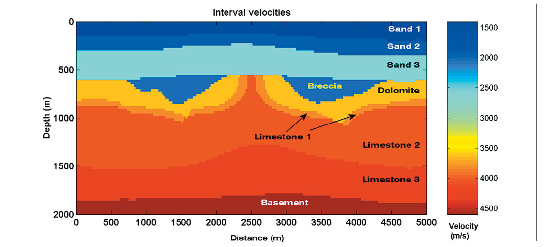
Figure 3 shows the geologic and velocity model I created. The model comprises all the summarized features present in real complex craters and has both vertical and lateral velocity variations. A cover of sands buries the structure to provide a flat surface for sources and receivers during ray tracing. The surface also served as a flat datum during data processing and thus no static corrections or velocity field manipulations were necessary.

Data Processing

I carried out the ray tracing in GX II with a Common Source simulation and a split spread geometry with both a shot interval and receiver separation of 50 m, along the total length of the model (5000 m). To generate the traces, the arrivals for each individual shot were convolved with a 256 ms Ricker wavelet having a dominant frequency of 30 Hz. The traces were 3500 ms long with a sampling interval of 2 ms. The generation process did not include geometrical spreading or seismic attenuation.

After ray-tracing and trace generation, I exported the data to Promax for further processing and migration. I also converted the interval velocities to RMS velocities for migration. All the migrations worked with a CDP interval of 25 m and maximum frequency of 80 Hz. The maximum dip migrated was 80 degrees.

Results and Discussion

I used Kirchhoff algorithms for all migrations because it is a reasonable algorithm for structured geology for its ability to handle both steep dips and laterally varying velocities (Promax reference manual, 1995; Kirtland Grech et al., 1998); features which are present in the crater model.

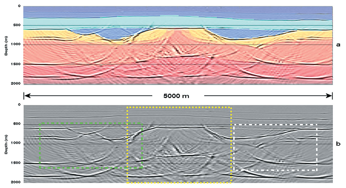
Figure 4 and Figure 5 show the two final post-stack and pre-stack depth migrations, respectively. In Figure 4a and Figure 5a the interval velocity structure overlays the migrated sections for reference. The first general impression is that both migrations have performed well in terms of general character and accuracy of positioning. In Figures 6, 7, and 8 I compare in more detail how the two migrations worked in the rectangular regions highlighted in Figures 4b and 5b. I discuss the most important results in the following sections.

Upturned steep layers and deep section (Figure 6)

Both depth migrations imaged relatively well the upturned layers of limestone 1 within the central peak (yellow arrows in Figure 6) The post-stack section (Figure 6a) gave a slightly superior result for the steepest parts of the model. These results confirm the ability of the Kirchhoff migration to handle steep dips (consider that in both cases the maximum dip migrated was 80 degrees).

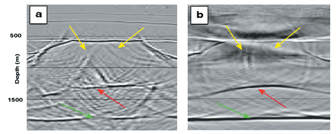
The pre-stack migration (Figure 6b) imaged very well the top of limestone 3 and the top of the basement, indicated respectively by red and green arrows in both figures. The post-stack migration also imaged these events at their correct position (Figure 6a), although the section is a lot noisier and has spread migration smiles.

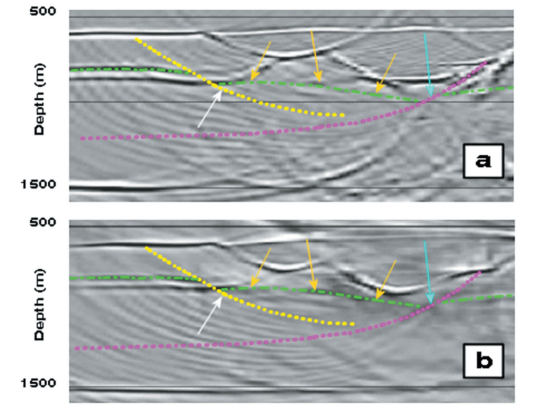
Sub-breccia events and fault planes (Figure 7 and Figure 8)

Figure 7 shows the results for the right-hand side of the model and Figure 8 those for the left-hand side. A number of events are less well imaged, some parts of the fault planes in particular (fault planes are indicated by dotted lines in both figures). However, the poor results are not caused by failure of the migration algorithms but they are due in most cases to the absence of acoustic impedance across part of the interface, where the same lithology is present in both the footwall and the hanging wall. On the other hand, where a lithology (and velocity) contrast is present either laterally or vertically, the fault surfaces are well imaged, as at the locations indicated by green and black arrows in Figure 7 and white and cyan arrows in Figure 8.

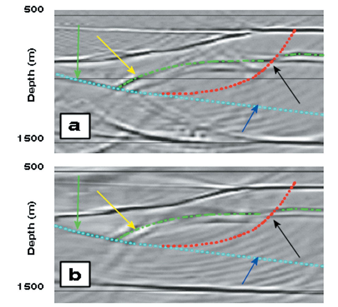
The orange arrows in Figure 8 indicate the area where the prestack migration yields better results than the post-stack migration in imaging the displaced top of limestone 1 (dash-dotted green line) below the left-hand side breccia deposit. In this regard, the shape of the low velocity deposit may have played an important role. Indeed, both migration algorithms performed well in imaging the top of limestone 1 below the right-hand side breccia deposit (yellow arrows in Figures 7a and 7b), where the deposit has a simpler shape. This suggests that a structurally complex lateral variation in velocity can affect migration results, although pre-stack depth migration seems to handle it better than post-stack depth migration (compare orange arrows in Figures 8a and 8b).

Post-stack TIME versus post-stack DEPTH migration

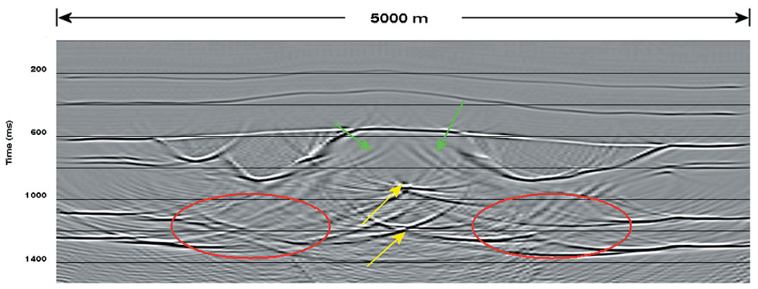
Figure 9 displays a post-stack time migrated section. Compared to the post-stack depth migration, the time migration has produced superior focussing of some events, in particular the upturned limestone 1 layers within the central peak (green arrows). However, the migration has performed poorly in the deeper section, especially in imaging the top of limestone 3 and the top of basement, both below the low breccia deposits (red ellipses) and at the apex of the anticlines (yellow arrows).

Summary

In this article I have compared the performance of different migration methods on synthetic data generated by modelling a complex impact structure. The model presented imaging challenges that are typical of these geologic structures. Both depth migrations imaged well the upturned, steeply dipping layers in the central uplift. Pre-stack depth migration imaged better the deep reflectors, especially in the most challenging part of the section below a complexly shaped low velocity breccia deposit. Pre-stack time migration produced superior results in terms of imaging the upturned layers in the central uplift but failed to image below the low velocity breccias.

Future Work

Experiment with the velocity model
Future work should include experiments to test velocity sensitivity with random variation of velocity of the geologic formations, migration with velocities obtained from conventional velocity analysis, inclusion of anisotropy in the geological model, and application of the results to data from real impact structures (e.g., Steen River crater, Northern Alberta).

Acknowledgements

I wish to thank Shauna Oppert, a former graduate student at the University of Calgary, for sharing with me her Promax expertise, hence contributing greatly to this study. I am indebted to Dr. John Bancroft for the many insightful lectures on migration and modelling of seismic data and for his useful comments during this research. I also thank Dr. Alan Hildebrand for teaching me a lot about impact craters. Finally, I thank Dr. Rob Stewart and Dr. Helen Isaac for their useful comments and suggestions, and for taking the time to read this article.