Migration Operator Aliasing and its Effect on Interpolation

Introduction

The controversial topic of 3D spatial sampling and its impact on the final seismic image has generated several articles in the last few years advocating coarsely sampled acquisition geometries (e.g. Neidell, 1994; Goodway & Ragan, 1996). On the other hand, Vermeer (1995) has advocated a fine, "symmetric" sampling geometry in 3D as an extension of his symmetric sampling ideas previously proposed for 2D acquisition (Vermeer, 1990). This article does not try to settle this debate in any way. It only deals with one of the finer details of migration (operator aliasing) which, unless understood, can lead to unnecessary confusion of the issues surrounding the larger debate. The following hypothetical storyline and data examples will illustrate the possible confusion that can arise when the effects of migration operator aliasing on coarsely sampled data are not understood.

A Good Idea that Leads to Puzzling Results

Suppose that you have been following the lively discussion between Vermeer and Neidell in The Leading Edge about 3D acquisition and the requirements for correct imaging (TLE, July, 1994; Sept., 1995). One point that Vermeer and Neidell did manage to agree on (among the many others that they disagree on) appeared in the September, 1995 TLE:

Neidell: The ultimate spatial sampling density (after migration) of the subsurface by the seismic survey is not tied to the bins as initially acquired in any prescribed or fixed manner.

Vermeer: (This statement) is 100% correct. The output sampling interval of migration may be selected as fine as you like it... However. it does not make sense to go to a finer sampling interval if the input data to migration is already aliased.

Satisfied that this statement must be true, since both Neidell and Vermeer managed to agree on it, you are anxious to put it to work in a way that can save money for your oil company, which acquires a considerable number of land 3D seismic datasets. Given that you have been of the opinion for some time prior to the Neidell and Vermeer publications that your data has been shot with too fine a poststack grid for the required resolution, you suggest using a coarser bin spacing (hence a coarser station spacing) to save costs. You have been using the standard bin size of 30m x 30m, and you suspect that it probably is not needed in order to image the structural dips that are being interpreted on your relatively unstructured datasets. Why not just acquire the data at a coarser bin size, say 60m x 30 m or 60m x 60m, and then obtain the desired bin size that the interpreters like by using migration to interpolate to a 30m x 30m bin at the end? The savings in acquisition costs could be substantial.

To test the idea, you take an existing 3D survey that has been shot with a 30m x 30 m bin size and decimate it to a 60m x 30m bin size. Kirchhoff migration is then used to interpolate back to the original bin size (the Kirchhoff algorithm allows the output to be computed at any location very easily). The result can then be calibrated against the original migrated data.

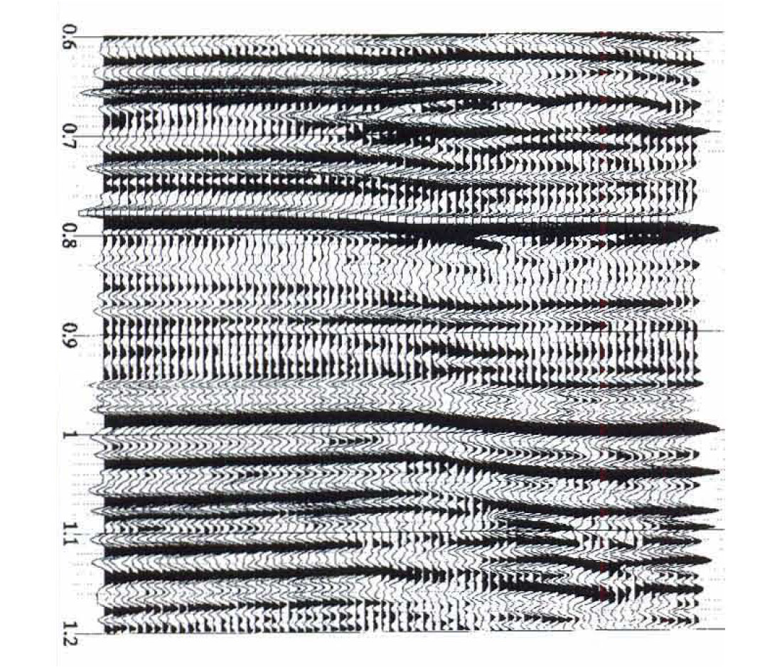
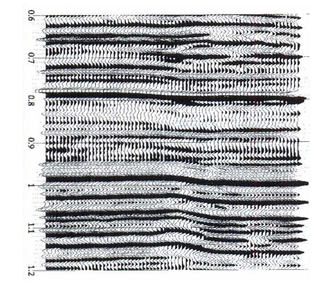
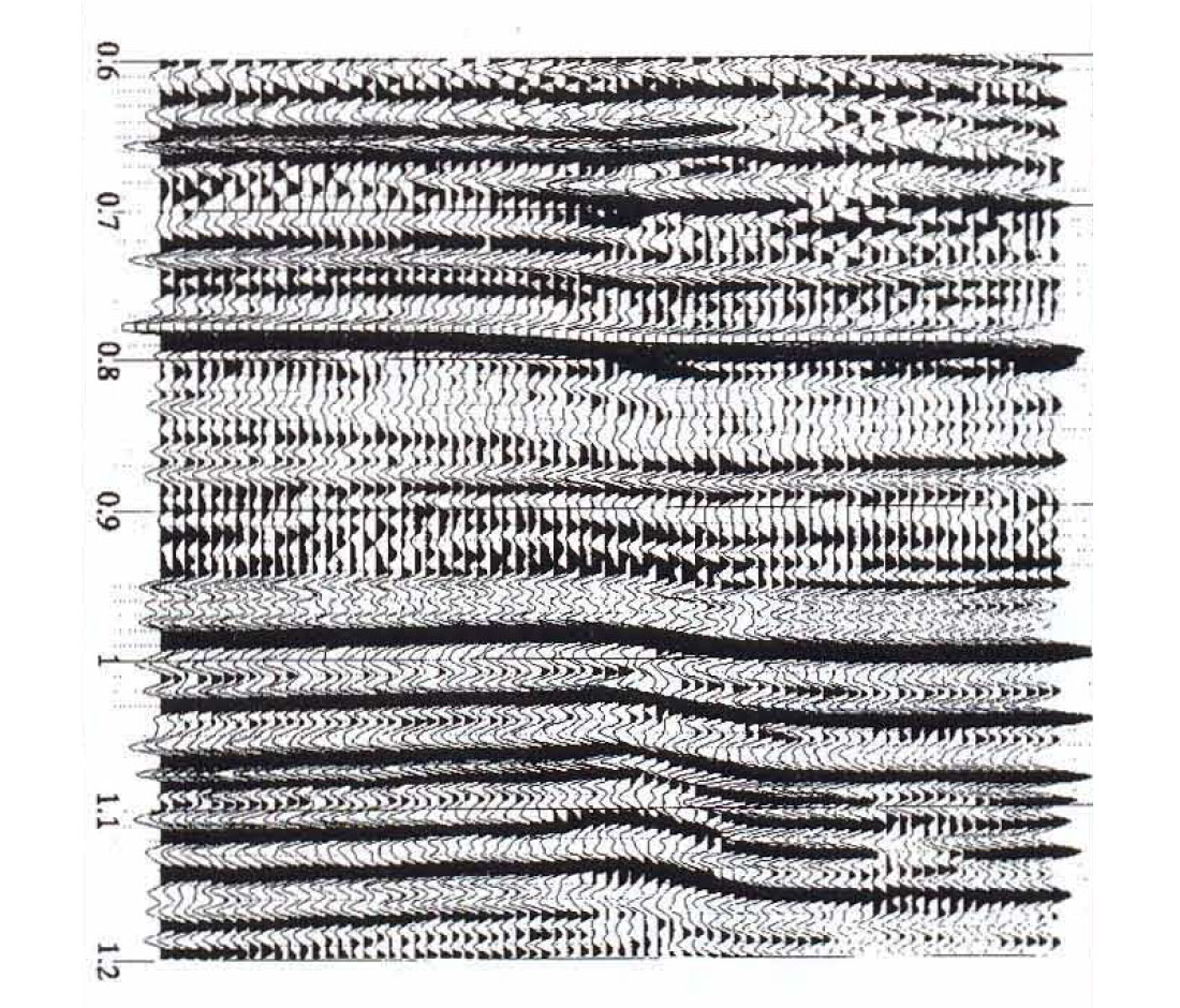
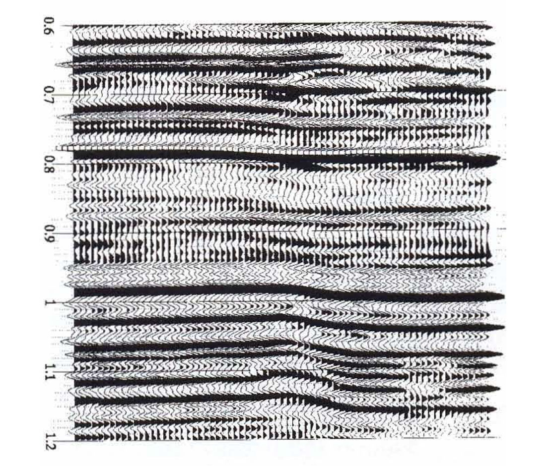
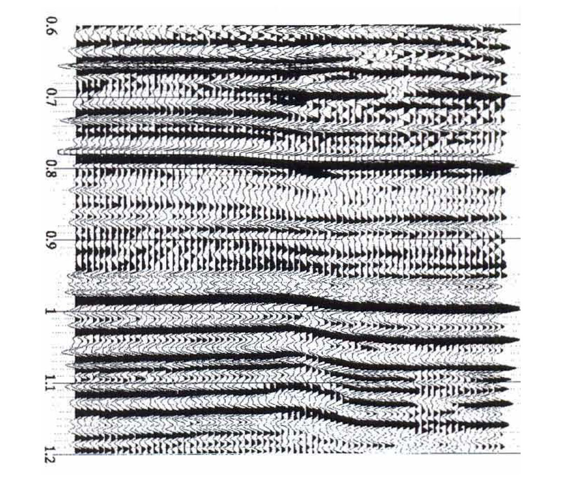
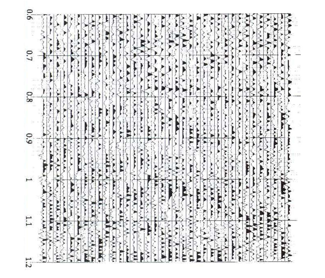
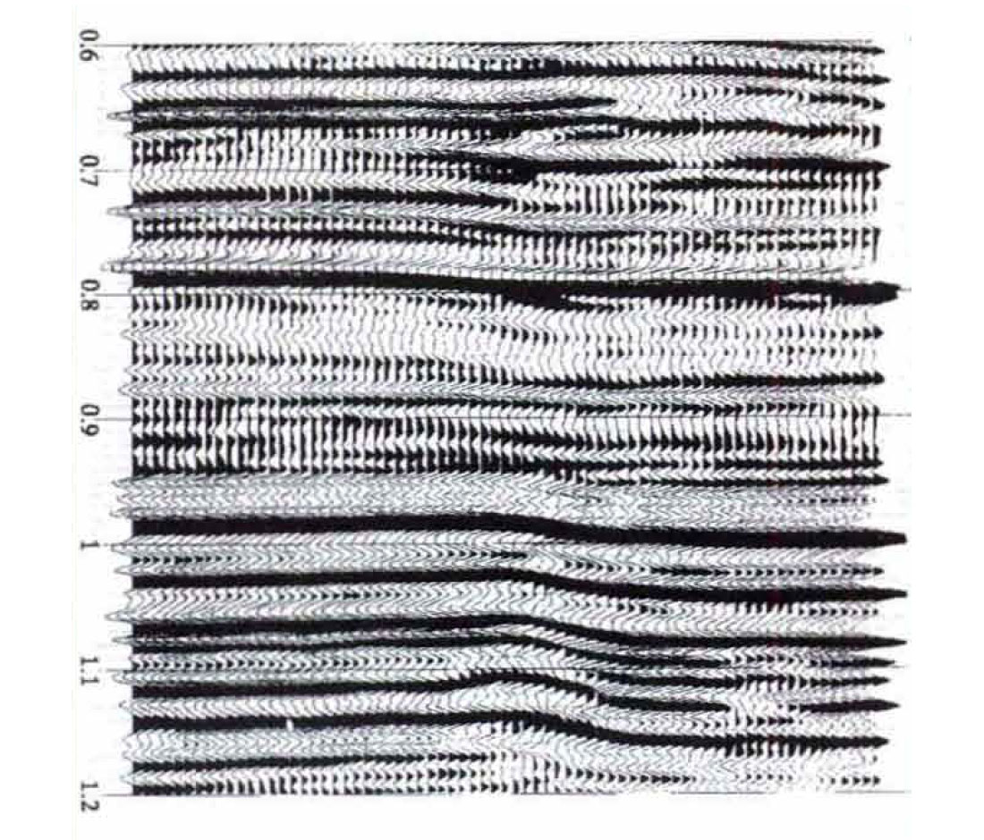
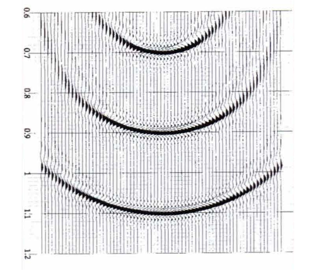
Figure 1 shows one of the inlines from the middle of the survey before migration at the original 30m bin size and Figure 2 shows the same line after decimation to a 60m bin size by zeroing every second trace. Figure 3 shows the 2D Kirchhoff migration of the inline shown in Figure 1, and Figure 4 shows the 2D Kirchhoff migration of the decimated data in Figure 2.

Obviously something is wrong. Instead of getting the same, or close to the same, result from the decimated data, Figure 4 shows a result that is obviously too noisy. What has gone wrong? You double-check everything-the velocities were the same for both, and the bin size was input correctly. The fact that a 2D migration was performed on the single inline instead of 3D migration cannot be the explanation either (a full 3D migration of the decimated 3D volume shows the same noisy result). Maybe it is something about the Kirchhoff migration algorithm that is causing the problem? But when you run finite-difference migration, you get the same result, as Figures 5 and 6 indicate. It also does not matter whether the dead traces are included as part of the input data or not the same result is obtained either way.

In frustration, you go back to double-check what it is that Vermeer and Neidell actually agreed to, and you re-read the qualifying statement by Vermeer:

... it does not make sense to go for a finer sampling interval, if the input data to migration is already aliased.

Perhaps this is the source of the problem: your decimated input data are aliased. However, the reason you thought you could interpolate the missing data with migration is because you predicted that the decimated data in Figure 2 would not be spatially aliased. In fact it still looks to you like the signal in the decimated data is adequately sampled at the 60m spacing, but you decide to do a test to check whether your eyes are playing tricks on you.

To test whether the signal in Figure 2 is aliased or not you perform a Fourier interpolation of the 60m data back to 30m. If the data are not aliased, then we should be able to reconstruct the data in Figure 1 from Figure 2 by going to the wavenumber domain, padding with zeros to twice the Nyquist wavenumber, and transforming back. If the data are aliased, this procedure will interpolate the data along aliased slopes, instead of along the correct slopes, and a poor interpolation will be the result. Note that some interpolation methods (e.g. Spitz, 1991) are capable of interpolating aliased data correctly by assuming that the data consist of a small number of linear events, but this type of method would not be able to tell us whether the data are aliased or not, which is our purpose here.

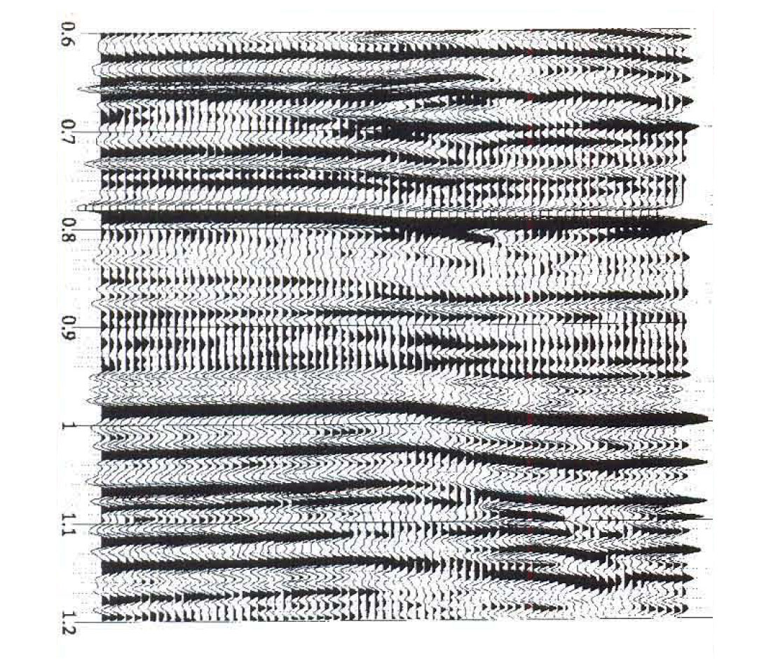
Figure 7 shows the results of the Fourier interpolation, and Figure 8 shows the difference between the data in Figures 1 and 7. The Fourier interpolation has worked well. The difference plot shows some hints of coherent events, but mostly the energy in this plot is from aliased noise. So this just confirms your suspicion that your data are not aliased at the 60m x 30m bin size, and that you have been overshooting your data at the finer grid size. But the problem of explaining the noise in Figure 4 still remains.

An Explanation for the Puzzling Results

Could it be that both Vermeer and Neidell are wrong? No, it just means that the issue is not as simple as it initially appears, and requires further explanation. The Fourier interpolation test points back to something about the migration as the cause of the problem since it is now known that the data can be interpolated with a method that adds no additional information (the Fourier method), migrated at the finer sample rate, and the correct result will be obtained. The problem is that the migration in Figure 4 was not performed in such a way as to interpolate the coarsely sampled data correctly.

The cause of the artifacts in Figures 4 and 6 is aliasing of the migration operator. Figure 9 shows the result of migrating the data in Figure 2 with a Kirchhoff migration operator that is correctly antialias protected. The migration now gives the desired result, which is almost the same as the migration result of Figure 3, but with half the input data.

Most geophysicists are familiar with data aliasing and can recognize it in their data where it occurs (e.g. Yilmaz, 1987, Section 1.6.1). Data that is aliased migrates incorrectly because the data is migrated along the aliased dips instead of the true dips. Operator aliasing is less familiar to many geophysicists, but can be just as important as data aliasing in many multichannel processes such as migration, DMO and Radon transforms (Hale, 1991; Lumley, 1994). Operator aliasing can be insidious: you can go into migration with data that is so flat that it hardly needs to be migrated, and yet your output will be degraded if operator aliasing is not accounted for correctly.

Figure 10 shows impulse responses of the migration operators that were used to generate the correctly migrated, undecimated data (Figure 3) and the incorrectly migrated, decimated data (Figure 4). The same (time-varying, spatially invariant) velocity function that was used to migrate the real data examples was also used to generate these impulse responses. Figure 11 shows the impulse responses of the migration operators used to migrate the decimated data correctly. Notice that the impulse responses have the same curvature and phase character in both Figure to and Figure 11. The only difference between them is in the frequency content of the steep flanks of the impulse responses. In both cases the frequency content of the wavelet on the impulse response drops as the angle (dip) increases, but the frequency content drops more rapidly in Figure 11 than in Figure 10.

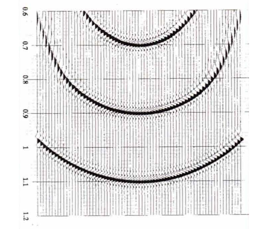
The rate at which the frequencies drop as a function of dip is governed by the spatial and temporal sampling rates of the data. The steepest dips in the data, either before or after migration, must be sampled at lea t twice per temporal wavelength and twice per spatial wavenumber if they are not to be aliased. Both the data and the migration operator must be governed by this aliasing rule in order to get an unaliased migration result. The wavelet at any given point on the migration operator should contain only frequencies that are unaliased for the slope of the operator at that point. Otherwise aliasing noise is introduced, even if the data are not aliased.

In summary, we can make the following statements about data aliasing and operator aliasing. Following Lumley et al.(l994), we consider input data aliasing, operator aliasing and image aliasing.

Input data aliasing:

If the input data to a process that involves spatial integration, such as migration, DMO or Radon transform, is spatially aliased, then the aliased components of the data will not be correctly processed. For example, an aliased plane wave will migrate along the aliased direction, instead of the correct direction. To get the correct result one can filter the aliased frequencies out of the input data and live with a lower frequency output, or else the filtering can be done in a dip-dependent manner during the process itself by changing the antialiasing protection of the operator to be more severe than it normally would be for the input data sampling rate. An alternative is to interpolate the data before input to a finer grid. Whatever interpolation method is used, it must work by providing some form of additional information to constrain the interpolation, since the data itself does not contain enough information about the wavefield. For example, Fourier interpolation, which adds no new information, will not work correctly when the data are aliased. However, f-x interpolation (Spitz, 1991; Claerbout, 1991) has the potential to overcome some of these costly acquisition Issues.

An obvious question arises from these statements about input data aliasing when we consider the ordinary NMO + stack process. Since the steep flanks of the reflection hyperbolas within a CMP gather are typically aliased before normal moveout, does the process of NMO + stack (a spatial integration process) give an aliased result?

The answer to this question must be no, because we are certainly able to preserve the high frequency content of reflections in our stacks. However, NMO + stack only gives an unaliased result when the velocity used for NMO is close to being correct. If the NMO velocities were so bad that the difference in slope between the reflections and the hyperbolic summation operator is beyond the two sample per wavelength aliasing limit, then the result would be aliased. A common example of aliased output from NMO + stack is the zipper pattern often seen in the shallow parts of stacks of marine data (e.g. Vermeer, 1990, Section 5.11.4). This odd/even effect is due to water-bottom multiples that are spatially aliased for the NMO + stack process, which is designed to image the faster velocity reflections. Examples of aliased output from NMO + stack of land data are provided by the linear, shot-generated noise that often leaks through the stack-array due to insufficient spatial sampling in the CMP domain, despite adequate shot sampling. Thus we have the sampling "paradox" pointed out by Vermeer (1990) and Jakubowicz (1994) and the K-filter spatial anti aliasing (Goodway, 1995) to remove the stack-array leakage.

Operator aliasing:

If the data going into migration, DMO or Radon transform are not aliased, then the output will still be aliased if the operator is aliased. The operator needs to be antialias protected according to the same sampling rule that governs the data: only plane-wave components that are sampled at least twice per spatial wavenumber are allowed on the operator at any point. The spatial sample rate of the input data governs the operator antialiasing requirements, not the output sample rate. The operator antialiasing criterion is a direct consequence of converting a line integral over a temporally and spatially bandlimited wavefield (i.e. a generalized Radon transform) to a summation over discrete samples of the wavefield.

Image aliasing:

The output data from the imaging algorithm may be aliased when neither the input data nor the operator is aliased. This situation can occur simply because the output sample rate is chosen to be too coarse to sample the output wavefield without aliasing. The output data can be sampled at any spatial interval, and if that interval is too large for all the dips in the data, the output is spatially aliased. This situation is simply avoided by calculating the output data at a finer spatial interval (e.g. the same as the input data sample rate).

Implications for Prestack Imaging:

The ability to successfully image seismic data with prestack processes that involve spatial integration like DMO and prestack migration depends on the prestack sampling of the wavefield. Exactly what the dependence is between 3D sampling and the final 3D image is the subject of the larger debate between Vermeer and Neidell, which is beyond the scope of this article. However, it is clear that operator antialiasing should be determined by the spatial sample rate of the input data volumes, which is often significantly worse than the spatial sample rate of the stack. Since operator antialiasing requirements impose a frequency-dependent aperture limitation on the migration operator, it is clear that the prestack data sample rate imposes a limit on the frequency content of dipping events that can be unambiguously processed through to the final image.

For example, for a 2-D line with an end-on shot every second station, the spatial sampling within each offset plane is one trace for every four CMP's. At this sample rate, the operator antialiasing requirements will severely limit the frequency content of the dipping events. If DMO or prestack time migration are to be applied with this coarse acquisition geometry, the options are either to stack offset planes together, which reduces the operator antialiasing restrictions but attenuates the dipping events during stack, or else to generate aliasing artifacts within each offset plane, and hope that the artifacts stack out while stacking all offsets together. Neither method will give perfect results. Only when very high-fold, and expensive, acquisition methods are used (such as "symmetric sampling", Vermeer, 1990), can the very highest quality results be guaranteed. Other acquisition geometries that rely on imperfect, but in some sense "adequate", cancellation of aliasing artifacts are currently under investigation (e.g. Zhou and Schuster, 1995).

It is important to note that all of the discussion of operator aliasing presented here has assumed a regular sampling grid. Since seismic data is almost always shot with some degree of irregularity in spatial sampling, an important question to investigate is the effect of irregularly sampled data on the final image.

Acknowledgements

We would like to thank PanCanadian Petroleum Ltd. for permission to present the data examples in this article.