Methodology for Seismic Inversion, A Western Canadian Reef Example

Abstract

Modern seismic inversion methods model both wavelet amplitude and phase effects and offer the opportunity for improved resolution and presentation of data in a form immediately recognizable to both geophysicists and geologists. This has re-focused our attention to the problem of non-uniqueness. Since the bandwidth of the seismic data is finite, there can be more than one mathematical solution to the seismic inversion problem. It has therefore become our task to differentiate between similar mathematical solutions on the basis of their geophysical and geological viability. Clearly, if this is to be done in an optimum way, all of the available information - seismic, logs, interpreted horizons and geology must be brought to bear upon the problem. To this end, we construct a 3D model of the project volume using the interpreted horizons and the logs. We then use the model both to constrain the inversion and to generate that low frequency component which is below the seismic bandwidth.

We focus not on the mathematics of the method itself, which have been described elsewhere (Debeye and Van Riel, 1990), but on the geological and geophysical constraints implicit in such an approach. We have previously viewed the procedure of wavelet estimation and seismic inversion as a part of the modelling process (Pendrel & Groeneveld, 1994). Our methods must be consistent with the model, be constrained by it and yet be flexible enough to detect deviations from the model which are the anomalies we seek. We establish constraints on the inversion to

• Limit the output impedances to a "fairway" of values about the log impedances.
• Set trace-to-trace variability constraints both in magnitude and arrival time.
• Control sparsity in the final inversion.
• Determine how low frequencies from the model are to be merged into the final inversion.

The result should be a seismic inversion which is robust and consistent with all the known information. We demonstrate this approach with a western Canadian example, a small 8600 bin 3D survey over a Devonian reef containing 17 wells, each with a set of sonic and density logs.

Introduction

The goal of seismic inversion is to transform the input seismic data to pseudo acoustic impedance logs at each CMP. More properly, then, it should be referred to as "inversion to acoustic impedance" although we shall use the shorter nomenclature here. The development of inversion methods which account for both wavelet amplitude and phase has resulted in an increased role for inversions as a diagnostic tool in the exploration for hydrocarbons.

The benefits of seismic inversion include

• Compensation for and reduction of the effects of wavelet tuning
• Presentation of output as geologic layers rather than reflection edges
• Merging of known low frequency geologic and geophysical information with seismic data
• Modelling and inclusion of layer stratigraphy
• Inclusion of geophysical constraints from known information or analogues.
• Calibration to well log data
• Improved interpretability of seismic horizons
• Increased bandwidth in the inversion output
• Attenuation of random noise

Inversion methods which account for wavelet sidelobe effects bring with them new problems. At first, it appears that our task might simply be to find a reflection coefficient series which when convolved with the model wavelet extracted from the seismic data, matches the input seismic data. However, since seismic data is band-limited, the solution to this problem is non-unique. Our challenge then is not to find an acceptable mathematical solution - in fact there are many - but to eliminate from consideration all those solutions which do not have geological or geophysical significance or which otherwise are not in agreement with known information. Since the inversion is meant to represent logs, we must also address the problem of estimating the low frequencies missing from the seismic data. This is done by extracting the lowest frequencies from a 3D model created from the logs and the interpreted horizons. The result will be a broad band inversion representing a set of pseudo acoustic impedance logs at each CMP. We present a methodology for doing this and demonstrate the procedure using data acquired over a Western Canadian Devonian reef.

Geology

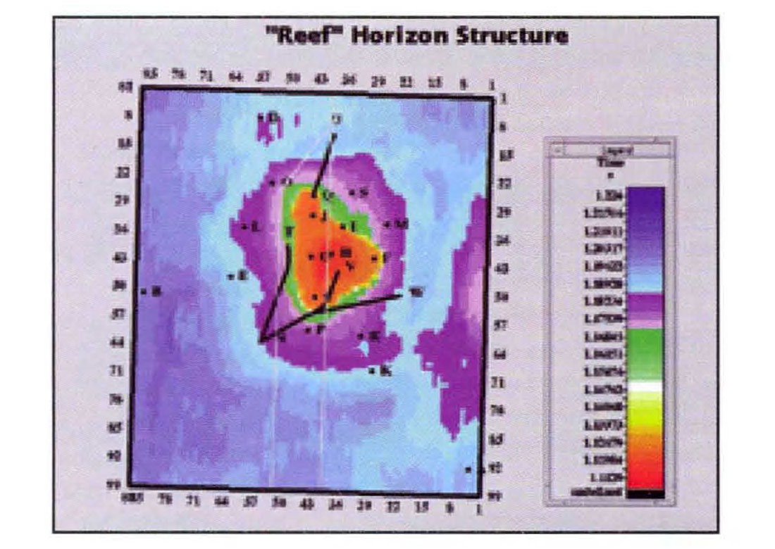
The geology is that of a Western Canadian Devonian reef. Figure 1 shows the reef structure and the locations of the wells used. The width of the main build-up is about I km. Surrounding the main reef build-up is a porous apron which away from the reef core interfingers with tighter facies. A lateral salt is present which is dissolved close to the main reef build-up. There were several episodes of dissolution. Some dissolutions were compensated by the basin material and some were not. This has had some influence in the small scale structure of the off-reef events. The off-reef basin facies are dolomitic and contain thin anhydrites which onlap against the reef. The considerable velocity contrast between the porous reef core and the high impedance off-reef facies has resulted in push-down of the reef platform and lower horizons. Other major reflectors are a shale-carbonate transition above the reef and a second deeper laterally continuous salt under the reef platform. Exploration issues centre around the distribution of apron porosity.

Methodology

Creating an Earth Model

The mathematics of the model have been described elsewhere and we will restrict ourselves to a largely non-mathematical description here. It is necessary to define the model structure in three dimensions. This is done by providing two pieces of information - the interpreted horizons and the model "framework". The framework, in the form of a spreadsheet, describes the ordering of the horizons in space and time and their behaviour at faults. The horizons, which can include interpreted faults. provide structure information, together, these form a 'blueprint' for the model. Stratigraphy within the layers is specified as onlap, offlap, reef, channel, etc. The model is completed by populating it with geophysical information, usually input in the form of well log data. We are most interested in impedance since this is needed to complete the low frequency portion of the seismic inversion. But in fact, we have also populated the model with other geophysical information - porosity, interval velocities from stacking velocities, etc.

The logs are usually provided in depth and the horizons in time. Thus it is necessary to create a time-depth transformation if these two pieces of information are to be rationalized. Input sonic logs are integrated, hung on an input time datum (one of the input horizons) and drift-corrected to tie the time horizons. Upon completion, the model exits in both time and depth and time-to-depth and depth-to-time transformations are possible.

Interpolation of the input log information between wells is done along layers, respecting both stratigraphy and faults. One of several simple interpolation schemes is generally used. They are more than adequate for the task of computing a low frequency background model for the sparse spike inversion. Quality control is done to ensure that well anomalies which might appear in the final inversion are not propagated throughout the model. Well masking and bandwidth control can be used to accomplish this. It is also possible to iteratively update the log interpolation function, driven by the need to achieve agreement between the synthetic implied by the model and the input seismic. In these inversions, the model, after iterative interpolation update and acceptable agreement between the synthetic and the seismic at each CMP, itself becomes the final inversion result. Inversions of this type will be the subject of a future paper.

Wavelet Analysis

Wavelet analysis is accomplished by computing a filter which best shapes the well log reflection coefficients to the input seismic at the well locations. The phase of the input seismic data, which may vary with frequency is found from the inverse of this filter. This wavelet, with amplitude representative of the seismic data, is input directly into the inversion algorithm or used to explicitly correct the phase of the input seismic to zero. If this latter route is chosen, then an equivalent zero phase wavelet must be provided to the inversion. This explicit correction to zero phase has the added advantage that spectral whitening can be done by specifying the correction bandwidth to be slightly wider than in the input seismic.

Constrained Sparse Spike Inversion

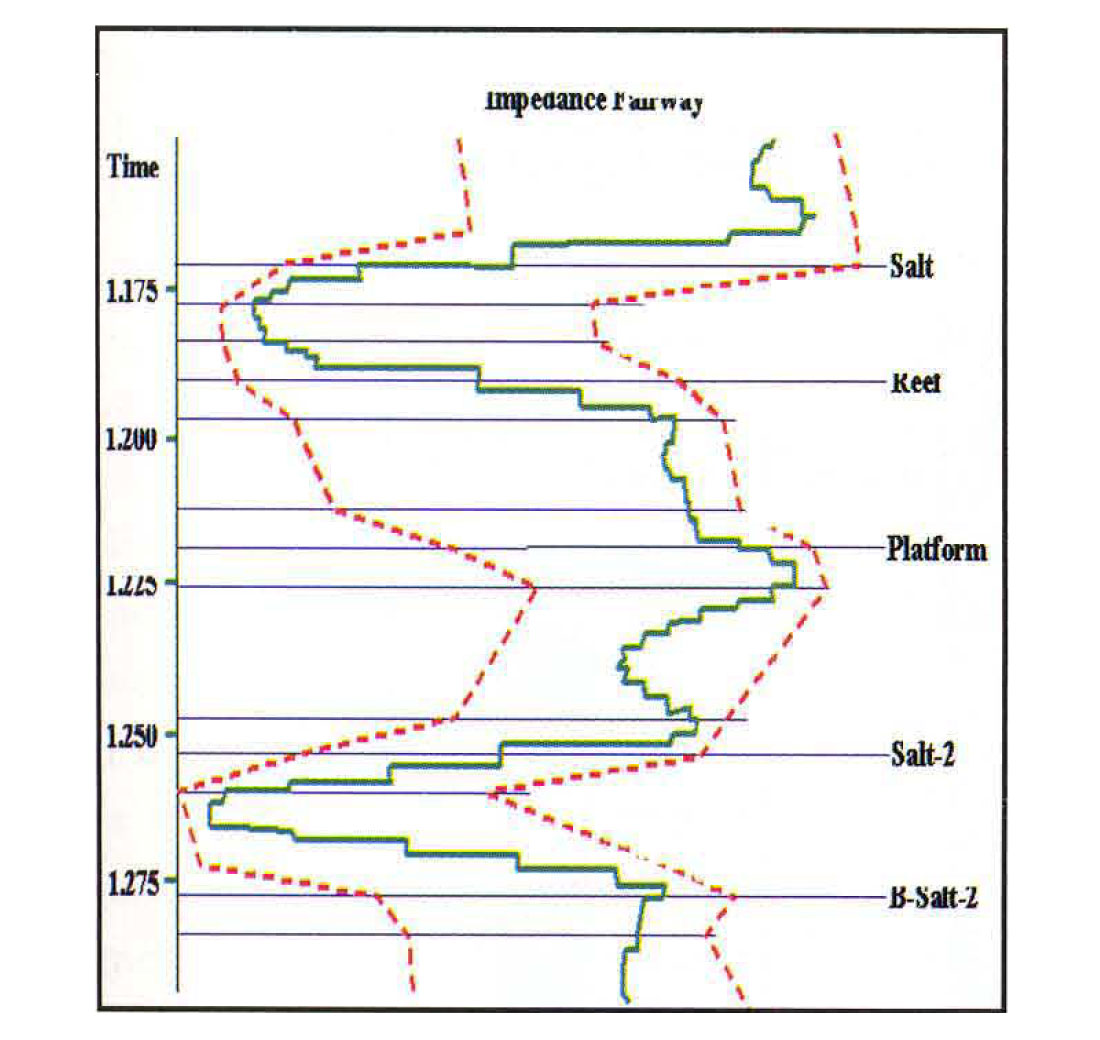
We seek to model the input seismic data as the convolution of the seismic wavelet with a reflection coefficient series. Because the seismic wavelet is band-limited, the problem is non-unique. There are many reflection coefficient series which when convolved with the seismic wavelet reproduce the input seismic to arbitrary accuracy. Thus, agreement of the sparse spike synthetic with the seismic becomes a necessary but not a sufficient condition in the solution of the inversion problem. To find the best geophysical and geological solution from the large number of available mathematical solutions, we must impose other conditions. These are provided by geophysical constraints which describe how the impedance can vary laterally away from the wells. A "fairway" of allowed impedances is defined, which limits the variability of inversion impedances and automatically rejects many good mathematical solutions which are geophysically or geologically not justifiable. The impedance fairway is conformable with the layering in the model and also has complete variability in time. These specifications force the inversion modelling problem to become non-linear, the solution to which is affected by an iterative technique. The number of iterations themselves, become a constraint, controlling the sparsity or blockiness of the inversion. Knowledge of the expected trace-to-trace impedance variations can also be provided to further limit the solutions. Since there is no guarantee in the mathematics that there will be agreement between the computed inversion and the impedance logs, quality control can be done by comparing them.

Acoustic Impedance Trace Merging

Although, the constraints in sparse spike inversion will guarantee the existence of low frequencies in the inversion, we do not expect that the information in the lowest frequencies will be reliable. This is a consequence of the band-limited nature of the seismic wavelet. The lowest reliable frequency will be project dependent, depending upon the quality of the input seismic and the constraints applied to it. Below this frequency, additional information must be provided. A "merge" frequency can be defined, below which, information in the final inversion is provided by the model. The model can be computed using logs from a single well or many, depending upon the circumstances. The former option will guarantee that no lateral varying information beyond that due to structure can come from the model while the latter will include the most available information about the project ,area. Above the merge frequency, information in the inversion comes from the constrained sparse spike output as described above.

Re-interpretation of Horizon Surfaces

Once an initial in version has been computed it is prudent to re-visit the interpretation. Since the inversion includes an automatic accounting for and removal of much of the wavelet sidelobe and tuning effects, the interpretation can be affected. Further, the inversion is in a "geologic" format as layers rather than reflection edges. If significant changes are made to the interpretation, then the model and indeed the inversion itself can be re-run.

Impedance Mapping

It is usually desired to measure and map anomalous impedance behaviour. This can be accomplished by computing the average impedance in a layer or layers conformable with one of the model horizons. Horizons conformable with any of the original input horizons are easily added to the model for this purpose. Flat horizons are a trivial simplification of this procedure. For the data presented here, we were interested in average apron porosity and its behaviour with depth below the apron. To this end, additional horizons conformable with the apron event were created.

Data

The project data consisted of 100 lines, each with 90 CMP's. The bin size was 40 * 40 m. Time migration before stack had been done and care taken to preserve true amplitudes.

Seventeen vertical wells, each with sonic and density logs were used. Computed porosity logs were available for many. Several horizontal wells were available for use as quality control. The key interpreted horizon was the "Reef' event which was picked along the top of the build-up until the salt was encountered whereupon the salt base was followed. Other key horizons were the shale carbonate interface above the reef, the reef platform and the tops of both salts.

It is always wise to spend some effort in quality control of the input data. We checked that the well tops were picked consistently and that they were "geophysical". By this we mean that they should be the well log counterparts of the interpreted horizons. Any necessary drift corrections were applied in the modelling step.

Results

EarthModel

A solid geologic model with a 2 ms sample interval was constructed from the well logs, interpreted horizons and a framework describing the arrangement of the layers. The framework was particularly simple since there were no faults and layers were built up, one upon the other. A section through the 3D model is shown in Figure 2.

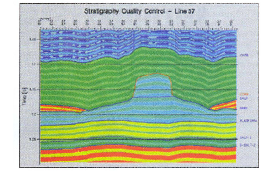
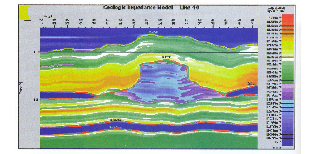
The broad colours are meant to indicate the layer boundaries. The structure of the finer banding internal to each layer is indicative of the stratigraphy. In most layers, the stratigraphy is conformable with the bounding horizons. Exceptions are the Salt layer which is conformable only with its upper boundary and the reef interior which has been defined to respect both the reef structure and the observed push-down. Figure 3 is the same section (line 40 - see Figure 1) through the final impedance model. Lateral variations in impedance arise from both structural and stratigraphic effects. At CMP's where no log is present, nearby logs were stretched or squeezed on a layer-by-layer basis to account for structure and then subjected to a weighted average to arrive at the model impedance. A simple distance-weighted average sufficed although the weights could have been set arbitrarily as required.

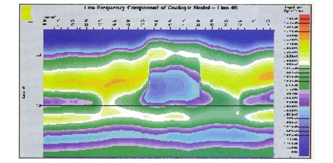
We used the model as a source of low frequencies in the final inversion. An example of a low frequency component of the model is shown in Figure 4. From this figure we see that the reef mass is a low frequency effect and that we will therefore need these frequencies if the reef is to be imaged correctly in the inversion.

Constrained Sparse Spike Inversion

Constraints were set within each geologic layer to limit the range of solutions to those which were geophysically admissible. These constraints, shown at well A in Figure 5, were assessed at each well and then extrapolated across the project area according to the model horizons. Note that we do not expect higher impedances in the Reef layer than those observed in the log. However, we do want to include inversion solutions which speak of lower impedances since we expect to encounter porosity. The impedance fairway reflects these beliefs.

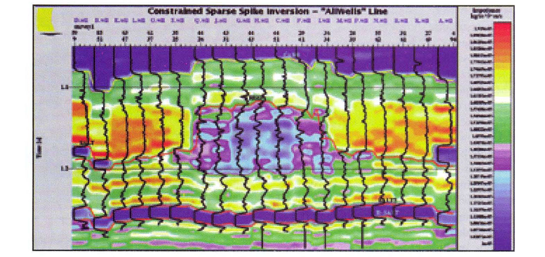
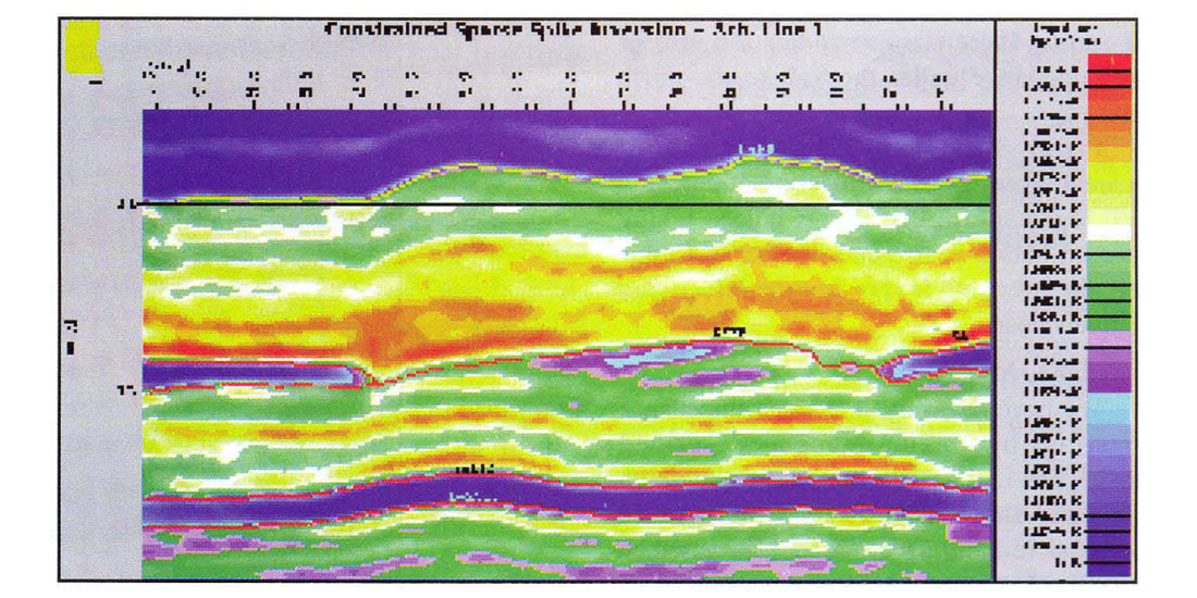
The final inversion along an "AllWells" line is shown in Figure 6 with the impedance logs superimposed. The disjointed nature of the plot is due to the distribution of the wells, although an attempt was made to proceed through the field in a somewhat orderly fashion. A good match with the superimposed impedance logs leads to confidence about the results of the inversion away from the wells. There is good agreement of the logs and the inversion in the salts and at the hale-carbonate interface above the reef. Sub-reef events are also well represented. The impedance change at the top of the reef core is gradual, emphasizing the need for low frequencies to correctly image the geology. Figure 7 is a section through the final inversion cube. The input seismic has been transformed to a layer domain. It now includes our best information about the low frequencies and the interpreted horizons. In fact, the horizons shown here were re-visited after a first round of inversion. The re-interpretation was done from the bandlimited (seismic only) component of the inversion. The model was then re-built and the inversion re-run. That is the result shown in the figure. Relatively low regions of impedance can be seen inside the reef core and in the apron. There is some indication also of low impedance under the Salt to the north (right).

Figure 8 shows an interesting case of apparent layering or interfingering of porosity. Well logs confirm that this is indeed taking place on both a coarse and fine scale. In this case, the inversion is showing the effect on a relatively coarse scale.

Impedance Maps

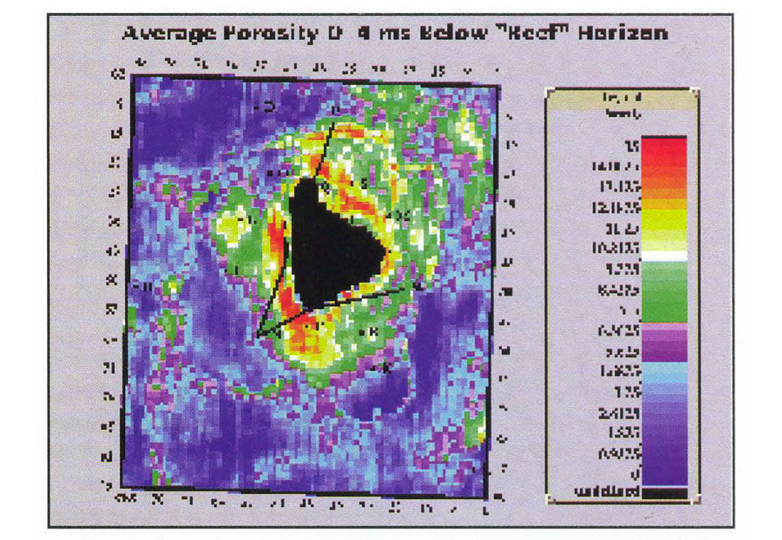
We have determined average impedance variations by making maps as described above. The reef apron event was copied both below and above itself. every ample for 20 ms. After re-building the model, it was then possible to measure the average impedance in anyone or combination of one-sample-thick layers. Since all of the layers were conformable with the apron horizon we could measure the lateral variation in average apron impedance. Figure 9 is a map for a sub-apron layer 4 ms thick, starting at the Reef event. Porosity development is evident to the south below well P, to the west at well L and to the north and north-west. The good porosity near the reef core is in agreement with the horizontal well observations.

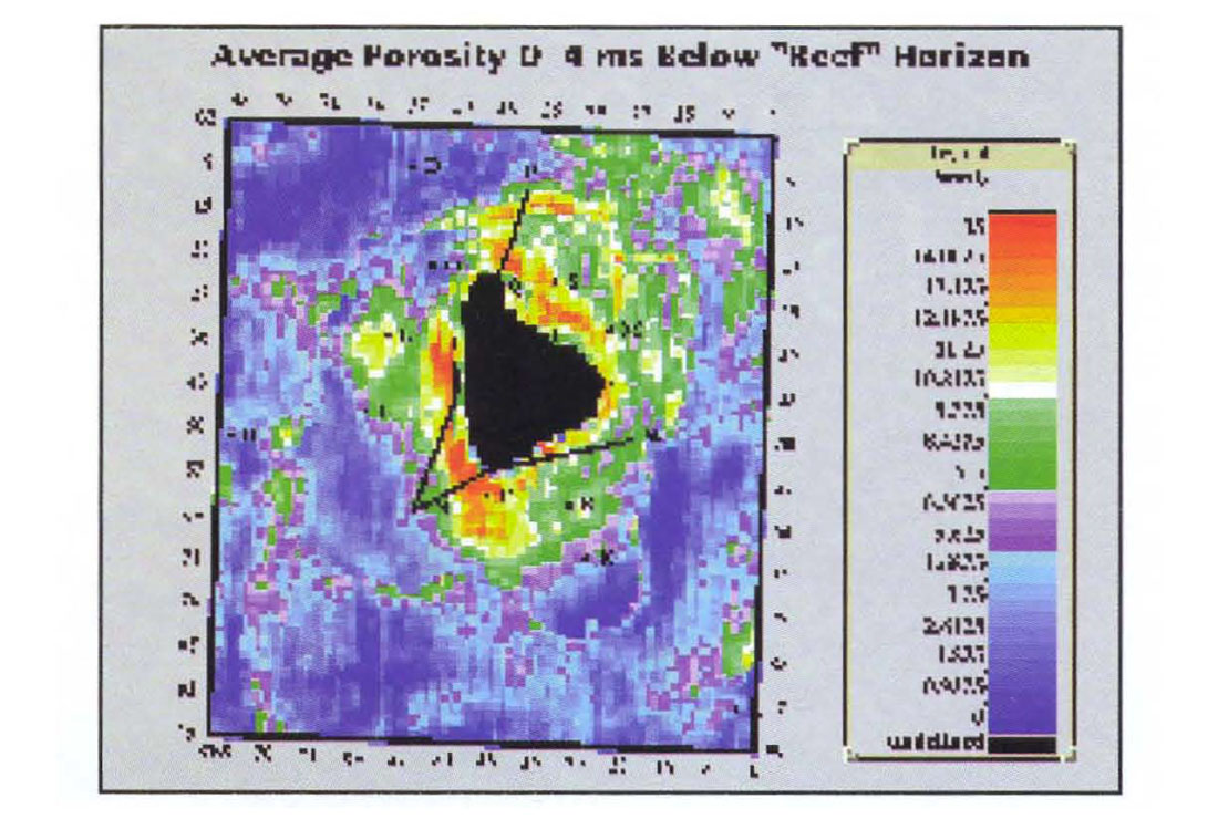
Figure 10 shows the average impedance in a deeper layer from 4 ms to 10 ms below the Reef horizon. The logs show decreased porosity with increasing depth below the reef apron and Figure 10 reflects this in the decreased impedance to the west, south and near-north. Farther to the north-west, the apparent porosity appears to have increased. However, this is partly a low frequency effect present in the model and we note that there is little well information in this region. In these data, both low and high frequencies are important. We do our best by the low frequencies in using all the logs to construct a geologic model. However, we can never know the low frequency component of the impedance precisely until a well is drilled. As more wells are drilled in the project area, the model will be upgraded. It is possible to make maps from the band-limited (seismic only) component of the inversion. In this case, there will be no low frequency component and no direct effects from the model. Since there will be both positive and negative numbers, we refer to this as a relative inversion. How the relative inversion correlates to average porosity is a project-dependent issue. Generally, we prefer to use reliable well log information when it is available.

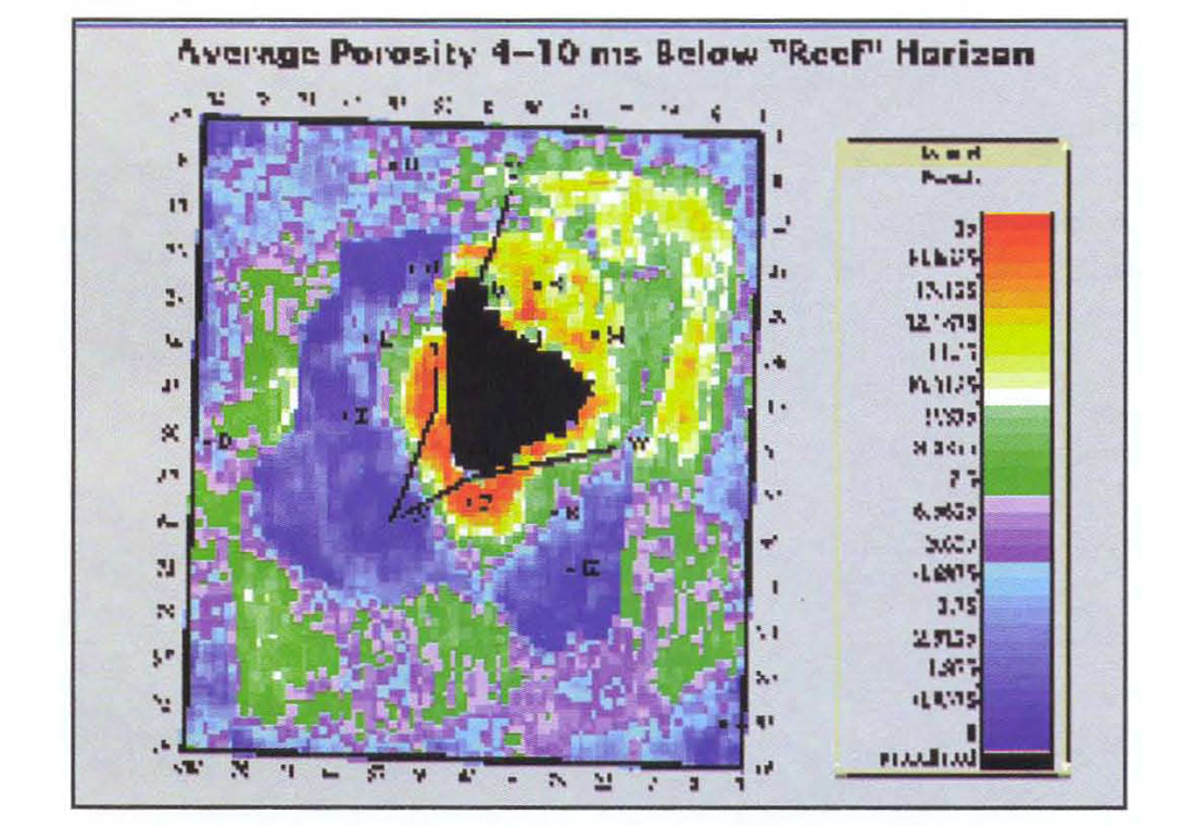
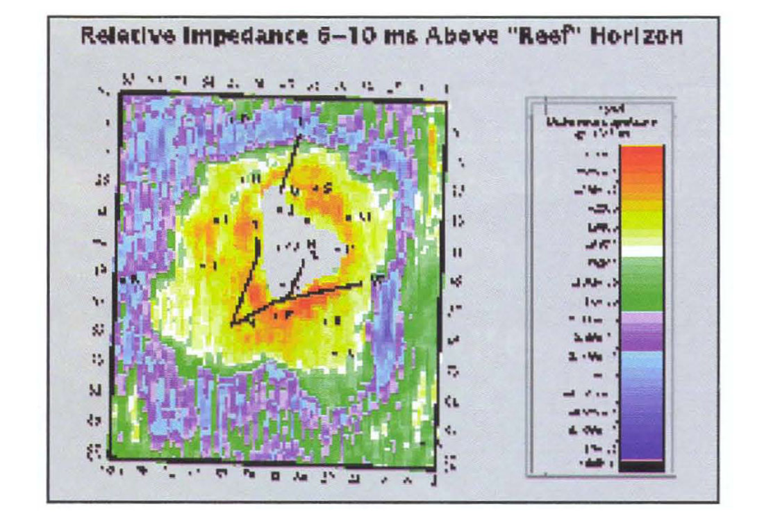
Figure 11 is an impedance map made from a relative inversion for a layer 4 ms thick, starting 6 ms above the apron event. It clearly shows the thin anhydrites against the reef build-up. Although not of exploration interest, these observations build confidence to our results generally, since they are in agreement with known geology.

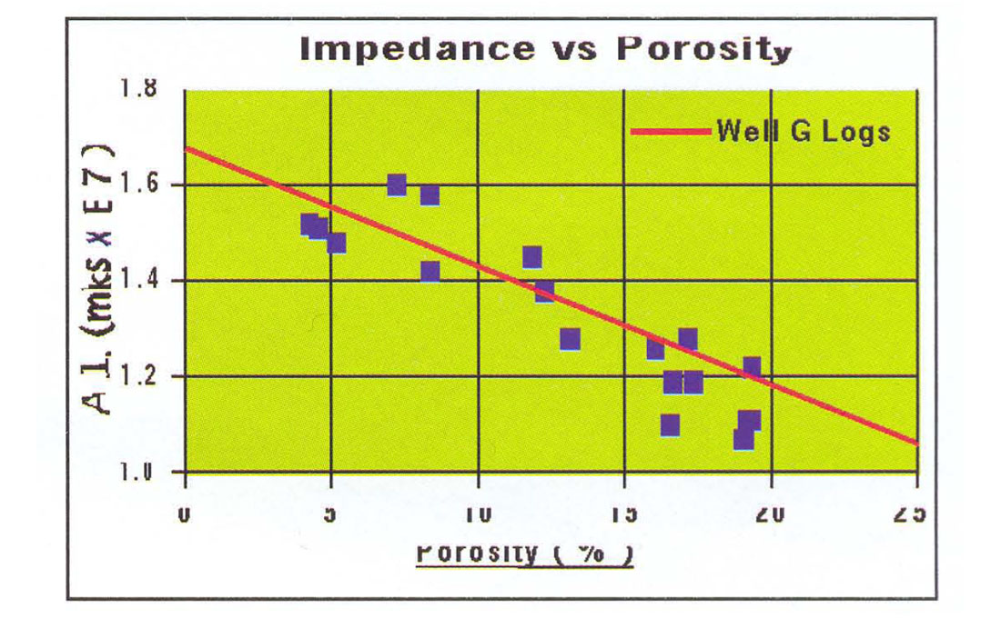
Porosity logs computed from neutrondensity crossplots were available at some of the wells. Corresponding average impedances were measured from the final inversion cube and the data plotted in Figure 12. Also shown is the best linear fit to impedance-porosity pairs from the Well G logs. The good agreement implies that valid porosities can be determined from the inversion. The average impedance in the thin layer immediately below the Reef horizon was converted to porosity and is shown in Figure 13.

Conclusions

Improved interpretability and understanding of the geology and geophysics in the project area has resulted from including all available information in the final inversion product. These have been in the form of seismic reflection data, interpreted horizons, and logs. It is not always possible that extensive drilling will have resulted in a thorough a priori understanding of the play. But when such knowledge is available, it should and here has been used to build an accurate and detailed model. One might at first be hesitant to build such models, especially in steeply dipping regions where we can guess that the seismic imaging has been less than perfect. However, we would be remiss in not using this available and accurate information from drilling. The fact that the seismic might not image these regions with accuracy simply means that we must attach a higher degree of uncertainty to it in these areas.

We note in closing that the modern seismic inversion is an ideal vehicle for bringing geologists and geophysicists together. The inversion is a geophysical product (albeit including some geologic information) but is presented in a form which is familiar to geologists. In this context, we have observed it to be the catalyst for many lively debates.

Acknowledgements

The authors gratefully acknowledge Husky Oil Ltd. and Mobil Oil Canada for their generous donation of these data.