Mechanics of Seismic Q

Seismic- wave attenuation and dispersion are studied in most geophysical curricular and broadly used in both academic and applied research. Applications of these concepts include identification of gas reservoirs and chimneys from frequencydependent seismic amplitudes, analysis of frequency dependent P- and S-wave velocities, interpretation of the effects of porosity and fluid saturation using laboratory experiments with rock samples, amplitudeand Q-variation with offset studies, time-lapse data analysis and reservoir monitoring, and Q-compensation increasing the resolution of reflection seismic sections. Attenuation effects are also included in many algorithms for waveform modeling, imaging, and full-waveform inversion.

Despite such long-established and often routine use, interpretations of seismic attenuation still contains several popular misconceptions about its nature. The key misconception consists in the core assumption that the energy dissipation rate in a wave-propagating medium can be described regardless of the physical mechanism, by a phenomenological property called the “Q-factor”. This material property was suggested from observations of rock creep in materials science (Lomnitz, 1957) and almost simultaneously introduced in seismology (e.g., Knopoff, 1956). This model describing the wave attenuation and dispersion by spatially- and (often) frequency-dependent Q-factors of the medium is usually called the viscoelastic (VE) model. However, already at that time, at the end of his famous paper entitled “Q”, Knopoff (1964) pointed out an important difficulty of the VE model for the Earth’s mantle. Unfortunately, the analysis of the physical consistency of this model was not pursued further at that time, and we need to continue it today.

The controversial subtlety of the concept of Q can be seen from the fact that it is used both as an observed quantity (measured in various experiments) and an in situ medium property (such as determining the frequency dependences of wave speeds). For example, by assigning Q values to thin rock layers, Qadrouh et al. (2018) recently compared several averaging formulas for layered media, similarly to averaging the density or elastic moduli. Measurements of the strain-stress ratios and phase lags for rock samples in the laboratory are often called “direct observations” of seismic attenuation and velocity dispersion (Batzle et al., 2014). In a study further considered in this paper, Pimienta et al. (2015) examine the empirical frequency dependencies of Q^-1(f ) for sandstone samples and identify the characteristic frequencies (“transitions”), which presumably also occur within these rocks at field conditions. However, note that if a material property denoted Q(f ) could indeed be measured so directly, this would be the only such case in physics! In physics, in order to determine some property of the medium (for example, wave speed), we typically have to measure some other quantities (such as distance and time in this case) and utilize the appropriate physical theories.

With regard to the seismic Q-factor, the understanding of its meaning and implications for modeling or interpreting seismic attenuation is still far from being sufficient. In the following section, I consider the physical meaning of the Q-factor by focusing on three general points:

1. Q is usually an empirical, or “apparent” quantity, which is specific to practically every type of deformation and experimental set-up an not simply related to material properties. This variability of Q is much broader than the usual differentiation of the Q-factors attributed to the bulk and shear moduli, or the differences between the “intrinsic” and “scattering” Qs. For example, Morozov and Deng (2018a) showed that the bulk-modulus attenuation (Q^-1) measured in a 8-cm long sandstone specimen by Pimienta et al. (2015) is about ten times greater than the Q^-1 measured in a traveling wave at the same frequency.
2. Although the VE model often leads to plausible predictions of decaying amplitudes and dispersive waveforms, such predictions are achieved phenomenologically by using the “correspondence principle” to insert the expected effective Q values into the “VE moduli” and wave equations. However, the correspondence principle is physically unjustified for waves, and particularly for porous rock (White, 1986).
3. Furthermore, the VE model is incomplete for heterogeneous media, which include practically all cases of interest in seismology. This model lacks boundary- condition relations for the internal variables on material-property contrasts. However, similarly to fluid-saturated porous rock, boundary conditions should often dominate the attenuation and dispersion effects.

The above arguments show that the Q model alone is often inaccurate and/or insufficient for describing seismic-wave attenuation, particularly when links to quantitative interpretation and geomechanics are required. In section “Mechanical approach”, I summarize an alternate, rigorous-mechanics based approach not relying on a Q.

Physical aspects of the Q model

There are numerous methods for measuring Q and its use in modeling and interpretation (e.g., Tonn, 1991). Each of these methods utilizes somewhat different aspects of the phenomenon of wave attenuation and dispersion and consequently produces a somewhat different “Q”. In this section, I identify six broad groups of Q-factors used in seismology and consider their relations to physics.

Six definitions of Q

Although conventionally denoted by the same symbol, at least six different broad definitions of the Q-factor can be recognized in seismic studies. When performing such classification, it is important to clearly differentiate between the measured (“apparent”) and true (in situ) properties (Morozov and Baharvand Ahmadi, 2015), and also to avoid “assumed” Q types and ad hoc simplifications. Note that this classification still does not include subdivisions of the Q-factors by wave types (P-, S-, surface-, or standing-wave) or types of recording (e.g., refracted or reflected waves), and consequently the actual variety of Q-factors is much broader.

First, I identify the “intended interpretational Q” as a parameter representing the general goal of attenuation/dispersion data analysis. This parameter is expected to be a phenomenological material property, defined so that its reduced values should be related to pores and fracturing, presence of fluids, elevated temperatures, and other factors causing internal mechanical friction or elastic scattering within the medium. This parameter is most valuable for the seismic interpreter or reservoir engineer, and it can be viewed as “true”. However, this Q is of course only the intended purpose of data analysis, and no single property of such kind likely exists in reality. The following Q-type quantities are therefore expected to be approximations for this “true” Q.

The second definition of the Q is standard in seismology texts (e.g., Aki and Richards, 2002) and originates from an analogy with a mechanical or electric resonator (oscillator):

However, this analogy is unfortunately invalid as the rock lacks the natural frequency f₀, which is the principal property of a resonator. For a resonator, the ratio in eq. (1) must actually be evaluated at frequency f₀, and Q^-1 represents the relative width of the spectral amplitude peak at f₀. It is easy to show that when applied to a forced oscillation at an arbitrary frequency f ≪ f₀ (such as in a low-frequency attenuation experiment; e.g., Batzle et al., 2014), eq. (1) would yield Q( f ) ∝ f . However, such frequency dependence of Q is nonphysical, because from the basic attenuation formula:

the seismic-wave amplitude then becomes frequency-independent A( f ,t) = A(t). This A(t) law basically represents a geometrical spreading, and no Q is needed for its description (Morozov et al., 2018a).

Thus, the Q defined by eq. (1) is “true” when applied to a finite body, such as in the measurements of free oscillations of the Earth (Knopoff, 1964) or resonant-bar attenuation measurements in the laboratory, but it is only “assumed” and not particularly useful when applied to traveling seismic waves or subresonant laboratory experiments.

Third, the Q-factor is often inferred from the viscoelastic (VE) theory, in which it represents the complex argument of the “VE modulus” in the frequency domain. For example, for the bulk modulus K:

and similarly for shear and other moduli. Similarly to eq. (1), this definition is “assumed”, as well as the VE model itself. Although leading to a (generally) consistent mathematical theory, the relation of eq. (3) to real rock can be unclear, particularly for fluid-saturated porous rock. In particular, White (1986) pointed out that the P-, S-, bulk- and Young’s moduli and the Poisson’s ratios for porous rock are not related as assumed in the VE model. This observation questions the data transformations utilized in many low-frequency experiments with porous rock (e.g., Batzle et al., 2014; Pimienta et al., 2015) and may present a serious problem for the conventional data analysis. Morozov and Deng (2018a) also argued that additional VE moduli and Q-factors similar to eq. (3) must be defined for Biot’s slow waves, and also for coupling between the fast- and slow-wave moduli.

The fourth definition of Q relates to from spectral measurements with propagating waves, such as by comparing the amplitudes A(f,t) in eq. (2) using the spectral ratio method (Tonn, 1991). Such Q can be combined with the phase velocity c to form the complex slowness (Aki and Richards, 2002):

This relation represents a form of the correspondence principle (next subsection). As combinations of empirically-measured quantities, these c, Q, and c* are “apparent”. An important consequence of this apparent character is that in order to measure either of these spectral quantities, substantial lengths of seismic records are required, and consequently the models for c and Q cannot be arbitrarily detailed spatially. This limitation of spatial resolution is significant; for example, White (1992) estimated that longer than ~100-ms records are required in order to measure a Q ≈ 100 with a modest 30% accuracy. In consequence of such inherent limitation of resolution, Morozov and Baharvand Ahmadi (2015) suggested that models for the apparent c and Q should better be always kept smooth in seismic data analysis.

The fifth definition is also observational (apparent) and arises from time-domain Q measurements often called the “single-station” method in earthquake seismology. In this method, the Q is estimated from the dependence of some measured frequency-dependent amplitude A(f,t) of a traveling-wave pulse corrected for geometric spreading G(f,t) (eq. (2)):

This empirical Q contains a significant contribution from the “assumed” dependence G(f,t). Note that generally, the geometric spreading can be highly detailed and frequency-dependent, although only simple frequency-independent forms of G(t) are usually considered in practice. Comparisons of many studies show that because of usually assuming straight rays, the decay rate of G(t) is often underestimated, leading to steep and spurious increases of Q(f ) with frequency f (Morozov, 2008, 2010).

Finally, in low-frequency laboratory attenuation experiments, yet another distinctive definition of Q is used:

where ϕ_ε and ϕ_σ are the measured phases of the harmonic strain and stress, respectively. More precisely, fs is measured as the strain of the elastic standard attached to the sample. Similarly to the above cases, the measurements of ϕ_ε and ϕ_σ involve experimental corrections, averaging and rely on simplifying assumptions, which also makes the resulting Q^-1( f ) “apparent”. In particular, Pimienta et al. (2015) showed that the low-frequency peaks of this Q^-1( f ) at f » 35- 600 Hz (for bulk deformation and water saturation at ~1 MPa differential pressure in sandstone) could be experimental artifacts caused by fluid penetration through the entire sample. Morozov and Deng (2018a) suggested a correction for this artifact which, however, still could not be removed completely.

In summary, the brief taxonomy above contains three definitions of “apparent” Q-factors that are different and contain significant subtleties and caveats. Only within the realm of the VE model, these apparent Qs can be reconciled together and with the two “assumed” types of Q. However, this model is insufficient for (at least) the most important case of porous rock, and consequently there is no common definition of Q that could reliably represent the internal friction within Earth media.

Correspondence principle

Let us now review how the internal friction is described in the VE theory, which is based on the “correspondence principle” (Lakes, 2009). This principle postulates that at any point x within a deformed body, the time series for stress σ (x,t) at any point x is partly delayed in time with respect to the strain ε (x,t), as given by the following relation:

where M(x,t) is the time-dependent VE modulus. Interestingly, the ε (x,t) is similarly delayed with respect to σ (x,t) regardless of the actual mechanism of interaction. This reciprocity of relations ε (x,t)↔σ (x,t') shows that eq. (7) is not really a causal physical law (for example, explaining how the stress is caused by strain) but only a mathematical identity relating the observed (apparent) time-dependencies of ε (x,t) and σ (x,t).

The time-only dependence of interactions ε (x,t)↔σ (x,t') (called “material memory”) with no interactions between ε (x,t) and σ (x,'t') at different points x and x' (eq. (7)) is another fundamental shortcoming of the VE model. In physics, the situation is opposite: there is no “memory” in time but interactions always propagate spatially by means of waves or transient processes such as diffusion. The ”material memory” at point x (eq. (7)) is thus apparent and consists, for example, of all direct and reflected waves passing through point x.

The hypothetical relation in eq. (7) is very flexible and allows obtaining almost arbitrary Q(f ) dependencies or creep functions (Lakes, 2009). However, some seemingly simple Q(f ) dependencies may actually require complex mechanical structures of the material. For example, the constant-Q attenuation, which is usually viewed as the “simplest” practical case, is particularly difficult to explain mechanically (Knopoff, 1956). Wave-equation models of constant-Q media require nonlinear attenuation mechanisms and additional material properties (Knopoff and MacDonald, 1958; Coulman et al., 2013). Band-limited approximations for near-constant-Q spectra are often implemented by multiple unobservable internal (“memory”) variables in the mechanical equations for the medium (Blanch et al., 1995). By contrast, the mechanically simplest case with no internal variables is given by viscosity, which is applicable to fluids, metals (Landau and Lifshitz, 1986), potentially heavy oil and some solids (Morozov et al., 2018b). The solid viscosity model yields Q( f ) ∝ f ^-1, and therefore such frequency dependence might deserve more attention in seismic studies.

Boundary conditions for internal variables

Because of the absence of spatial interactions in eq. (7), the VE model also disregards any non-VE wavemodes and any forces acting on the internal (“memory”) variables near material-property contrasts. Nevertheless, in wave mechanics, non-VE modes should exist (Morozov and Deng, 2018b). In contrast to, for example, slow P waves in Biot’s poroelastic model, skin depths for non-VE modes are infinite (Morozov and Deng, 2016), and consequently these modes should effectively couple even with widely spaced boundaries.

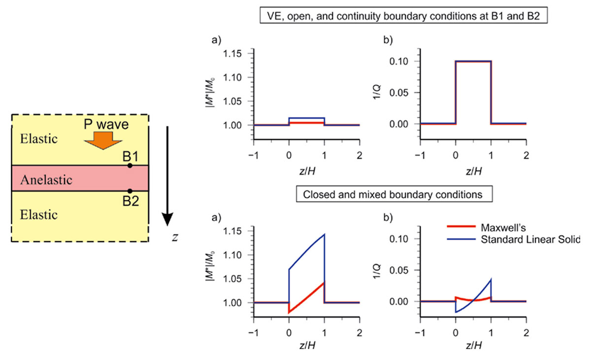
With the present limited knowledge of the mechanics of internal friction, it is difficult to determine how the non-VE wave modes should interact with material-property contrasts, but we should definitely not exclude such interactions a priori. Figure 1 compares the effects of the usual “open”, “closed”, and continuity boundary conditions on the internal variables modeled for a single anelastic layer enclosed between two elastic half-spaces. Similarly to the constraints on cross-boundary pore-fluid flows in poroelasticity (Dunn, 1987), ”closed“ boundaries almost completely suppress the observed (apparent) attenuation (Figure 1). Also note that the resulting Q^-1 is spatially variable across the anelastic layer, and it can be negative for Maxwell’s rheology of the layer. These results are not expected in the VE model but naturally follow from wave mechanics.

Mechanical approach

As shown in the preceding section, Q is an insufficiently welldefined property in order to be used for detailed, accurate, and reliable modeling of rock anelasticity. At the same time, rigorous approaches to the mechanics of solids, fluids, and many other areas of physics are well known (Landau and Lifshitz, 1986). Here, I use such a formulation, called the “General Linear Solid” (GLS) by Morozov and Deng (2016). Owing to its generality, this formulation incorporates many of the existing first-principle models for rock and wave-propagating media: the poroelastic model by Biot (1962), several of its extensions (e.g., Deng and Morozov, 2016), doubleporosity models, and also all physically-realizable VE models.

In the GLS approach, the dynamics of a medium or a rock body is described by its Lagrangian function L (usually a combination of the kinetic and elastic energies) and the dissipation pseudo-potential D if the medium is lossy. For linear elasticity and internal friction, the most general forms of these functions are dissipation pseudo-potential D if the medium is lossy. For linear elasticity and internal friction, the most general forms of these functions

where V is the volume of the body, spatial coordinates are indicated by subscripts i and j, summations over repeated indices are implied, and superscripts ^T denote the matrix transposes in the N-dimensional model space. Model vector u is the displacement vector, in which the first element is the displacement of the representative volume element (RVE) of the rock. The rest of the variables correspond to internal degrees of freedom, such as filtration-fluid displacements or memory variables in a VE model. The bulk strain Δ and deviatoric strain ɛ̃_ij are derived from displacements u by standard differential relations. The N×N matrices Κ,  comprise material properties describing its elasticity (bulk and shear, respectively), matrix d describes the internal friction proportional to RVE velocities, matrices η_K and η_μ represent the viscous friction proportional to strain rates, and ρ is the density matrix specifying the inertial properties of the material.

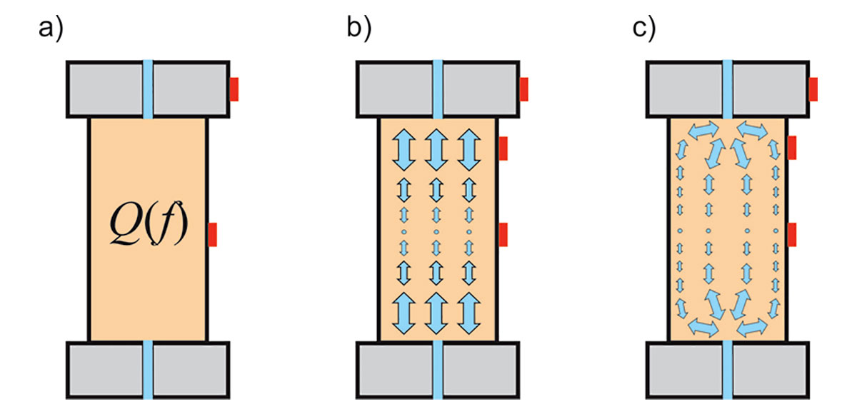
Despite its compact form, model (8) is complete and rigorous, and it allows straightforward derivation of all equations of motion and boundary conditions (Morozov and Deng, 2016). Most importantly, model (8) uses only time- and frequency-independent material properties to explain the frequency-dependent observations. Another key lesson from the mechanical approach is that each experiment must be modeled with precise and specific detail including the size and shape of the sample, the heterogeneity of the pore flow, the elastic standard, and placements of strain gauges (Figure 2). Simplistic assumptions about a “Q” of the material and uniform stress and strain fields (Figure 2a) may lead to incorrect results for wet porous rock (Morozov, 2015). With realistic pore-flow patterns through the end platens of the sample, the deformation becomes non-uniform, and the attenuation is concentrated within the “skin layers” near the ends of the sample (Figure 2b) or near fluid injection points (Figure 2c).

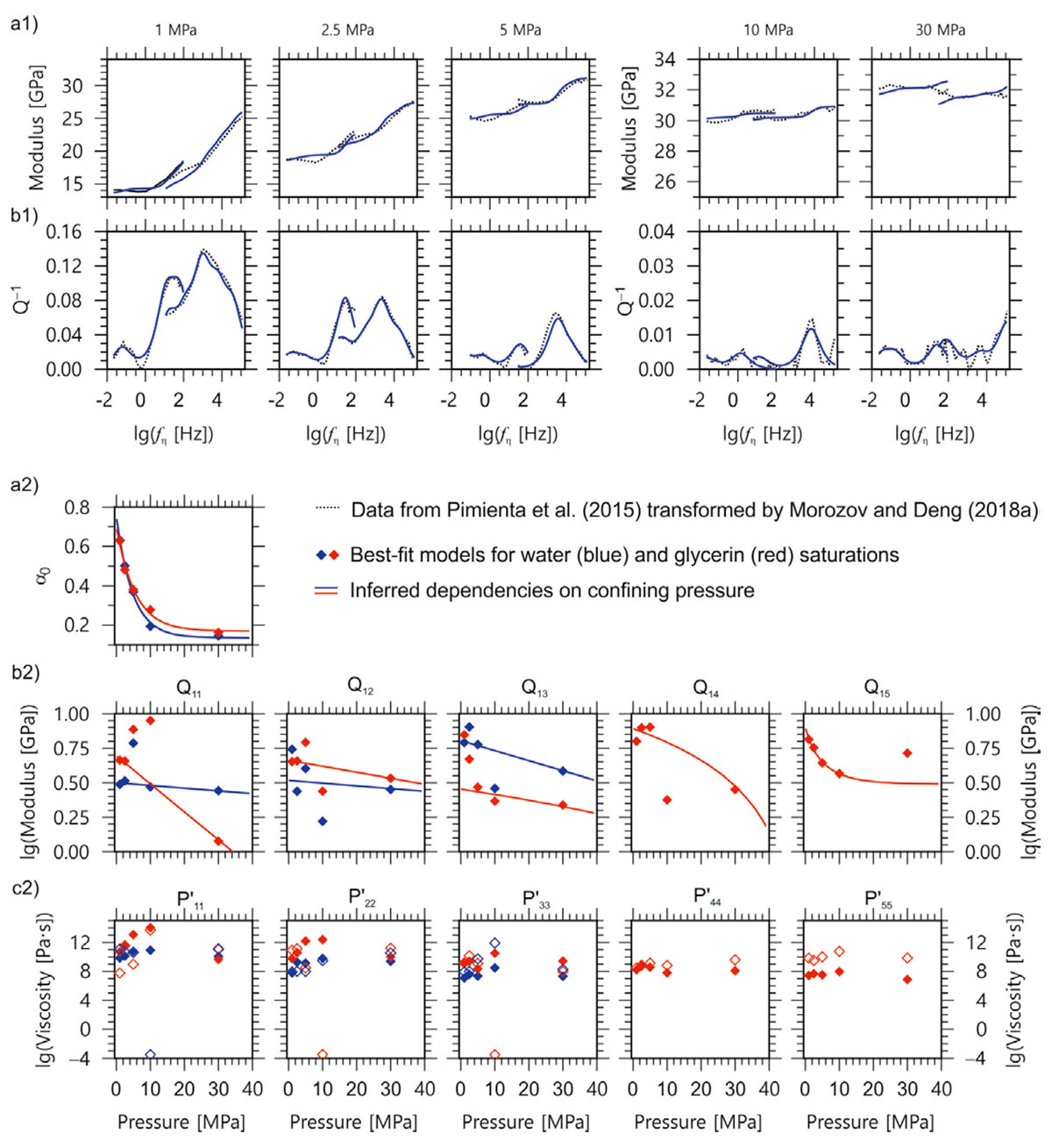
The GLS approach similar to eq. (8) allows modeling laboratory attenuation experiments with adequate detail and accuracy. In the model shown in (Figure 3), a 1-D approximation is used for deformation (Figure 2b) with a slightly different parameterization using scalar internal variables representing dilatations of Biot’s poroelastic frame. The elastic coefficients of this model are denoted by matrix Q (analogous to Κ in eq. (8); not to be confused with the apparent Q-factor), and the viscosity matrix is denoted P' (Figure 3, bottom). Five internal variables allow predicting the data closely (Figure 3, top) and reveal quantitative and unambiguous mechanical properties of the material (the Biot-Willis coefficient α₀ and elements of matrices Q and P') at variable confining pressures. These properties can be used to perform reliable finite-difference simulations of seismic wavefields or to model arbitrary mechanical experiments with this material. The mechanical model (eq. (8)) also contains the effects of permeability and should be suitable for geomechanical modeling, for example, of pore-fluid flows within the reservoir.

Conclusions

The conventional seismic Q-factor measured in field and laboratory experiments is usually an apparent quantity, which often depends on the types and parameters of the experiments. The viscoelastic model is also inaccurate for fluid-saturated porous rock, which is of primary interest in exploration seismology. By contrast, methods of continuum mechanics lead to rigorous, quantitative, accurate and detailed modeling of the behavior of rock in any laboratory and field environments.