Long–spreadlength approximations to NMO function for a multi-layered subsurface

Introduction

Conventional approximations of the NMO function assume a modest offset/depth ratio. Similarly conventional velocity analysis uses a hyperbolic approximation for the reflection traveltimes:

Here t₀ is a zero-offset time, x is an offset and V_RMS is NMO velocity. It is worth mentioning that velocity analysis does not give us an RMS velocity. The RMS velocity is a velocity defined by a mathematical formula (see formula (14)) and the NMO (stacking) velocity is a velocity from the hyperbolic approximation of an actual non-hyperbolic NMO curve, t(x). Even in theory, they are equal only for the homogeneous subsurface with a horizontal boundary. For any different subsurface model, the NMO velocity is not equal to the RMS velocity. However, in many practical cases, for example the vertically heterogeneous subsurface with conventional spreadlengths close to the reflector depth, the NMO velocity is close to the RMS velocity. Then we can use the NMO velocity as a reasonable estimation of the RMS velocity. At the same time, we should remember that these two velocities represent different notions and have different meanings.

With increasing offsets of up to double the reflector depth and greater, the hyperbolic NMO function exhibits errors in the reflection traveltime approximation. The hyperbolic NMO approximation does not fully account for velocity analysis and stacking of long-offset reflection data. Non-hyperbolic NMO approximations have been considered in many papers (Al-Chalabi, 1973, 1974, Malovichko, 1978, Blias, 1982, Goldin, 1986, Castle, 1994, Alkhalifah and Tsvankin, 1995, Taner et al, 2005). Instead of the conventional two-term hyperbolic approximation, a three-term approximation is proposed to improve NMO representation and to lead to a more accurate RMS velocity estimation. Since an exact NMO representation can be written only in a parametric form, all the proposed explicit NMO functions are approximate. A higher- order term NMO approximation enables a more accurate approximation of the observed travel times, but different NMO functions have different limitations with respect to the spreadlength/depth ratio.

An NMO formula is an approximate equation that connects offsets and traveltimes. Using more than two terms improves its accuracy, but at the same time creates some problems for velocity estimation. Adding an extra parameter leads to a more expensive velocity analysis and increases the RMS velocity variance by approximately 10 times. This was noticed by Al-Chalabi through random modeling (1974, fig. B3) and can be proved analytically. Because adding a fourth term again increases RMS velocity variance about 10 times, from a practical point of view the maximum number of estimated coefficients for one gather should be 3. For long offsets (offset/depth ≈ 1.5 – 2.5) we can expect significant improvement of V_RMS estimation using a three-term velocity analysis, even though it leads to a larger standard deviation.

For the longer offsets, three-term approximations do not correct travel times and sometimes residual corrections are needed. Some of the functions need fewer corrections and some need more. In this paper, we describe an approach for an approximate NMO formula derivation. Three new NMO formulae are derived using this approach. We test the accuracy of known NMO approximations as well as the new ones on different model data.

There are two main problems with respect to the NMO function application. The first problem is connected with the accuracy of this function as an approximation to the observed travel times. The second problem is connected with velocity inversion and interval velocity estimation using the Dix formula or its generalization. For horizontally stratified media, the accuracy of the interval velocity determination is directly connected with the accuracy of the RMS velocity estimation. Using different models, we will investigate both problems for the known and new NMO formulae.

Method

The traveltime function t(x) can be expanded into a Taylor series of x². It was first done by Bolshih (1956):

where

where h_k is a thickness of the k-th layer and v_k is its interval velocity; n is a number of layers above a reflector. He gave formulas for the first four coefficients a_k in terms of interval velocities and indicated that all coefficients a_k might be derived one at a time (one after another). Taner and Koehler (1969) suggested representing t² as a series expansion of x²:

Equations (4) can be obtained by squaring equation (2), which gives:

When the above is combined with (3), we obtain:

Formula (4) is more accurate than formula (2) since for a one layer model, (4) gives exact times for t(x) while (2) remains as an infinite series. For the long offsets, the hyperbolic approximation (1) is not accurate enough. Because the exact formula for traveltimes is an infinite series, many authors have proposed some improvements to the hyperbola, using more than two parameters. In this paper, we will derive several new three-parameter NMO formulae and compare different approximations.

Equations (2) or (4) enable us to find derivatives of time t or t² with respect to x² at x = 0:

There are different forms of approximations, proposed by several researchers, but the main idea of all NMO approximations is to keep time t and its two derivatives at x = 0 the same as the exact travel time function t(x).

Let’s consider any three-term approximation of the NMO function

where F is a function of four variables; a, b and c are the NMO parameters, x is an offset. To calculate coefficients a, b and c, we have to solve the system of three equations with respect to a, b and c:

where a₀, a₁ and a₂ are determined by (3). From the system (*), we can determine a, b and c and find the explicit approximation (2). The main problem here is to choose the function F(a,b,c,x) so that we can find the explicit solution of the last system.

Different NMO approximations

Let S be a dimensionless parameter, defined by the formula

We will consider the three-term approximation (4). Using parameter S, we can rewrite the three-term approximation (4) as:

For a homogeneous medium, S = 1. The greater the heterogeneity, the larger the value of S, so we can consider the difference (S-1) as a measure of the vertical velocity heterogeneity. Malovichko (1979) derived a representation of NMO in the form of a shifted hyperbola:

His derivation was repeated by Castle (1994) using the same complicated approach with Gauss’s hypergeometric series. It was used by Blias (1982) to develop a generalization of Dix formula for long offsets. Equation (8) can be derived using system (3). For this, let’s find an NMO approximation of the form:

where ξ = x²; a, b and c are coefficients to be determined. To find these coefficients, we find the first and second derivatives with respect to ξ at ξ = 0:

After substituting ξ = 0 into these equations and taking into account that t(x=0) = a₀, we obtain the system of three equations with three unknown parameters a, b and c:

This system can be solved for the unknown a, b and c, which leads us to formula (8).

The expression (8) is more accurate than (7) because for large offsets (i.e. as x tends to infinity) it behaves as x, the same as the exact traveltime function, while (7) behaves as x², while the factor g corresponds to average and RMS velocities, which is more convenient from practical point of view. Let us also consider a three-term NMO function similar to Alkhalifah and Tsvankin (1995). Using system (*) we come to the NMO equation for an isotropic medium:

Taner et al. (2005) considered NMO representation in the form:

where “a” is defined as an acceleration factor. System (3) for this approximation leads us to the solution for the coefficient a:

Let us consider another approach to the NMO equation, using the average velocity. For a homogeneous medium with velocity V, V_RMS = V_Ave = V. For this medium instead of (1), we can write:

where V_Ave is an average velocity given by

where H is reflector depth. For a layered medium, this NMO formula should be corrected for the vertical heterogeneity. For this, let’s consider a rational function

with an unknown coefficient “a”. To find coefficient “a”, we use the last equation (*), which leads to solution:

where g is a vertical heterogeneity factor, suggested by Al- Chalabi (1973, 1974):

The heterogeneity factor g is equal to 0 for homogeneous media. Thus, it is a measure of the vertical heterogeneity, in addition to the parameter S. The difference between the parameter S and the heterogeneity factor g is that S connects first and third moments of interval velocities, while the factor g corresponds to average and RMS velocities which is more convenient from practical point of view.

We can improve (11) by using an additional term. After some mathematical transformation, using an approximate formula

we obtain another NMO approximation:

Because the RMS velocity is connected with the average velocity and the heterogeneity factor g (formula (g)), the last formula also actually depends on three parameters: t₀, V_Ave and g.

Let us consider another NMO function in the form:

Using the same approach, and based on system (*), we come to the NMO expression:

Accuracy of different NMO approximations

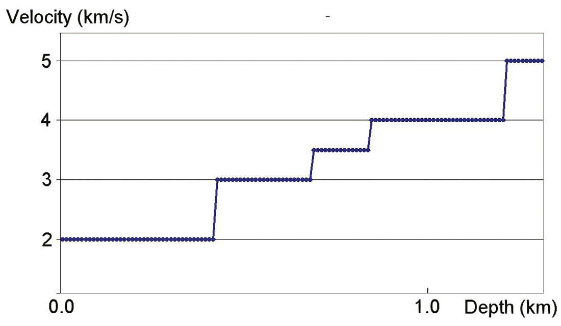
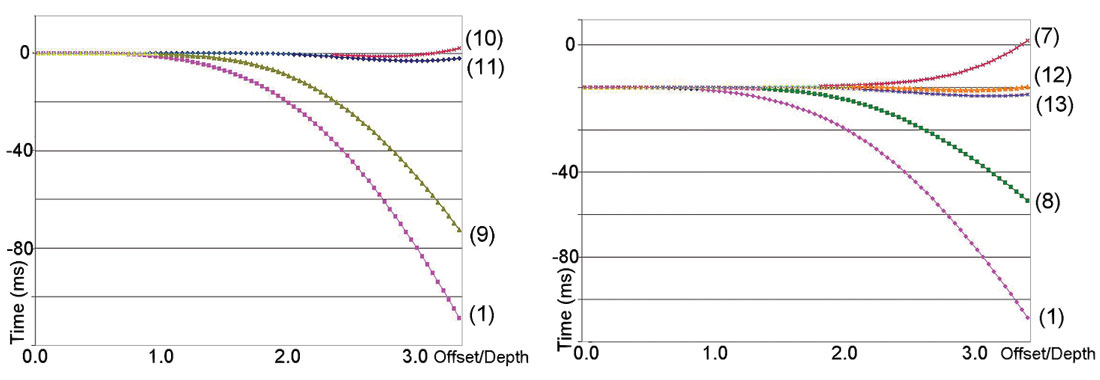
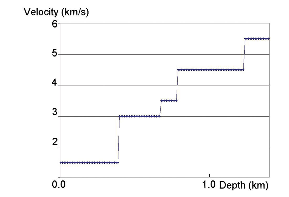
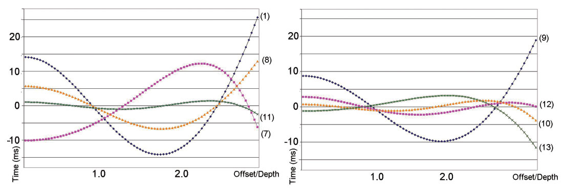
All of the NMO functions (7) – (13) were tested on different depth velocity models. All of them show that expressions (10) – (13) have the highest accuracy for long spreadlength. For example, let’s consider a layered depth model with moderate vertical heterogeneity (g = 0.103, S = 1.408) (fig. 1). For this model, I calculated the NMO functions using hyperbola (1) and equations (7) – (13). The exact NMO function was calculated through raytracing, and the residual traveltimes were computed for each NMO approximation. Figure 2 displays the approximation errors. Comparing the different NMO approximations with respect to residual moveout; which affects the quality of stacked data, for the offset/depth less than 1, all the approximations are accurate enough. The new approximations (11) – (13) and the approximation (10) fit the exact traveltimes very well at large offsets up to 3.5 x depth.

The least square approximations for three-term velocity analysis

Here we consider the accuracy of the various NMO functions as an approximation to observed travel times for a three term velocity analysis. To investigate the errors of each NMO approximation to fit actual traveltimes, we used several models with different heterogeneity. Even for the models with a large vertical heterogeneity and offsets up to 3 times reflector depth, the new approximations (11) – (13) were observed to fit the actual NMO curve with a high degree of accuracy. Figure 3 displays a depth velocity model with large vertical heterogeneity (g = 0.255, S = 1.88).

For this model, we calculated NMO functions through raytracing. Each NMO approximation (7) – (13) was used to approximate the NMO curve using the least-squares method for three parameters. Figure 4 shows the residual NMO time for the spreadlength equal to 3 times reflector depth. We see that even for this depth velocity model with large vertical heterogeneity, equations (10) – (13) fit the exact NMO curve very closely. For the spreadlength/depth less than 2.0, the approximation error of these approximations does not exceed 1 ms.

RMS velocity estimation

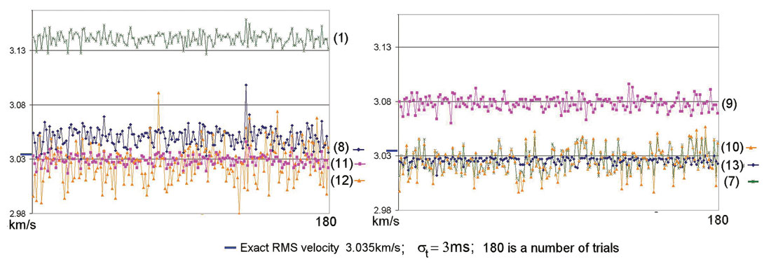
All the above NMO approximations can be used to estimate the RMS velocity through three-term velocity analysis. All of these equations represent different RMS velocity estimations with different statistical properties. Each of these formulae correspond to an NMO approximation that can be used in velocity analysis. For fixed t₀, each NMO formula (except hyperbola (1)) depends on two parameters. We can estimate the RMS velocity using NMO formulae (7) – (13) by performing three-term velocity analysis. Because all the formulae are approximate, these estimations will be different with respect to VRMS bias and standard deviation. To investigate the accuracy of RMS velocity estimation using different NMO approximations in the presence of random noise, we simulate the scenario with random time shifts (Al-Chalabi, 1974). To test the various NMO approximations, we used the model as shown in Figure 1. Traveltimes were calculated using raytracing, and a random time jitter with standard deviation of 3 ms was added to the NMO functions. I then determined three coefficients of each approximation using the least squares method for the spreadlength equal to two reflector depths. Figure 5 displays the result of 180 trials. We see that formula (11) and formula (13) give the most accurate estimation of RMS velocity.

Depth estimation

Conventional NMO functions provide us only with an RMS velocity but not the average velocity. For the vertically heterogeneous layers, the Dix formula gives us an estimation of the RMS interval velocity but not the average interval velocity. By RMS velocity we mean velocity as defined by formula (Taner and Koehler, 1969):

where 't_k is a vertical one-way time in the k-th layer. Average velocity V_Ave is determined by formula:

where H is a reflector depth and T is the one-way vertical time. If an estimated layer is heterogeneous (includes several horizontal layers) then Dix formula estimates RMS interval velocity in this layer but not average interval velocity (Al-Chalabi, 1974). The difference between RMS and average velocities in the layer is described using the heterogeneity factor g, (recall formula (g)) (Al-Chalabi, 1974). The heterogeneity factor g is always positive (0 for homogeneous layer) and can be as large as 0.1 (and greater). For a highly heterogeneous layer, the difference between the interval velocity, estimated through the Dix formula (that is interval RMS velocity) and average interval velocity may be as great as 10%, and possibly more. It may lead to significant errors in the depth estimation as made with Dix interval velocities even if the RMS velocities were obtained with very high accuracy.

Two new NMO expressions (11) and (12) refer directly to the average velocity instead of the RMS velocity.

It implies that this average velocity can be estimated directly from a long-offset velocity analysis, using these NMO representations. This enables an estimate of average velocity from long-offset velocity analysis, and thus the determination of reflector depth with more accuracy. This implies that we can determine a reflector depth using average velocity instead of RMS velocity, and it might lead us to a more accurate depth estimation from seismic data. Formulae (11) and (12) can be rewritten using reflector depth H and the heterogeneity factor g:

Each of the above NMO approximations include three parameters: t₀, g and H, which can be determined through three-term NMO analysis. Using these formulae, we can consider three-term velocity in terms of the depth H, zero-offset time t₀ and the heterogeneity factor g.

To test this approach to depth estimation, a depth velocity model was created from real sonic log data. Figure 6 shows the depth velocity model with high velocity layers, which affect the Dix velocity estimations and cause significant differences between average and RMS interval velocities. For the approximations (1), (7) – (10) and (13), the RMS velocity was estimated through three-term velocity analysis for five reflectors at the depths 0.5, 1.0 1.5, 2.0 and 2.5 km. Subsequently the Dix formula was applied to estimate interval velocities and thickness for each of the five layers. The reflector depth was estimated as the sum of five layer thicknesses.

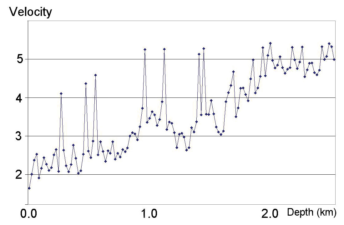
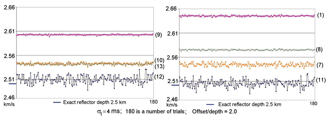
Figure 7 shows depths as estimated from the different NMO approximations for the spreadlength equal to 2 times the reflector depth for 180 trials with the added standard deviation of random NMO time jitter of 4 ms. This figure shows that expressions (11) and (12) give the most accurate depth estimation.

Conclusions

We have presented an approach to derive several different NMO approximations for horizontally stratified isotropic media. This approach is based on keeping time t(x²) and its first and second derivatives with respect to x² at offset x = 0 the same as for exact NMO function. Three new NMO functions have been derived and tested on model data together with the known ones. The new approximations appear to be the most accurate in terms of residual traveltimes and RMS velocity estimations, particularly at large offsets. Two of the new NMO approximations include average velocity as one of the parameters. This enables an estimate of reflector depth directly from velocity analysis rather than depth estimation through the Dix formula and RMS velocities.