Limitations of Deterministic and Advantages of Stochastic Seismic Inversion

Limitations of Deterministic Inversion

Inversion techniques to estimate impedance from seismic have been available to geophysicists for over twenty years. Conventional methods are referred to as ”deterministic” and are based on the minimisation of an error term between the forward convolution of the reflectivity from an estimated impedance profile and the seismic amplitudes at each trace location.

Due to its limited bandwidth and in particular the absence of low frequencies it is not possible to directly recover absolute impedance from a seismic trace. All inversion schemes with an absolute impedance output therefore require a constraint. This constraint or prior information is usually obtained from interpolation of well impedance logs and guided by picked seismic horizons. After inversion this prior information is embedded in the resulting absolute impedance estimates. Since the background impedance model is uncertain and so interpolated between the wells it may introduce artefacts which can be misleading in subsequent interpretation.

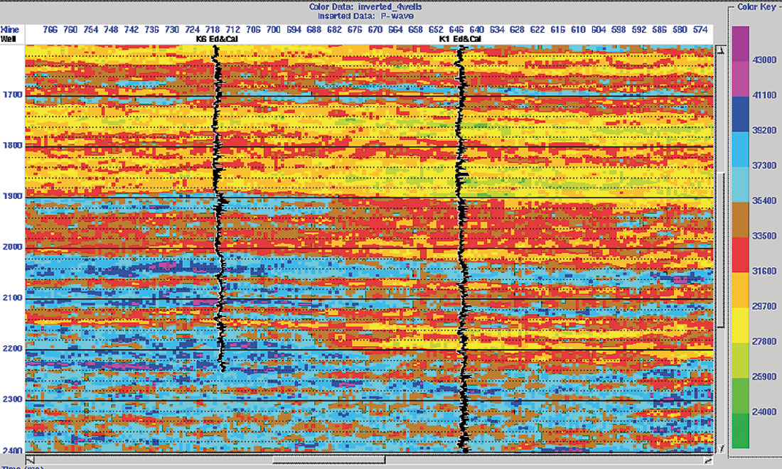
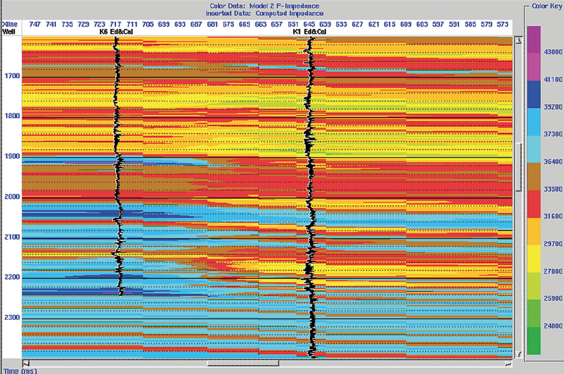
Two examples of this problem are shown here. The first is taken from Francis and Syed (2001) and is shown in Figure 1. In this example the reservoir sands in the inversion result appear to terminate between the K1 and K6 wells. The sands are low impedances (yellow/green) in the interval 2150-2200ms. Examination of the prior model (bottom panel of Figure 1) shows that this is an artefact caused by the initial model.

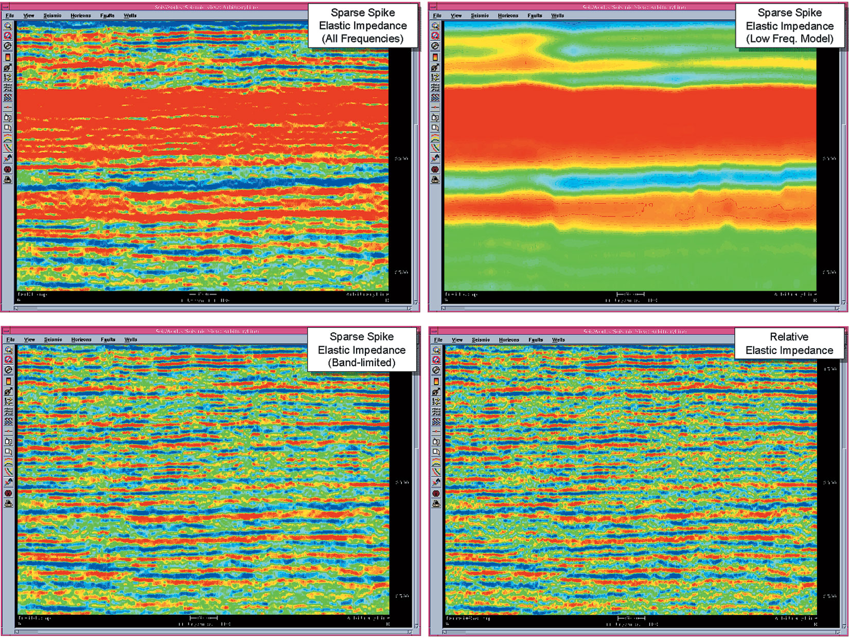
Some inversion schemes amount to little more than a relative impedance from the seismic added to a low frequency model. This can be demonstrated by filtering the low frequencies out of the inversion result and comparing with relative impedance. An example is shown in Figure 2. A commercial sparse spike inversion algorithm was used by the contractor to compute absolute elastic impedance (Figure 2(a)). By applying a low pass filter, the low frequency model is seen (Figure 2(b)), with artefacts caused by three well locations clearly visible. A high pass filter reveals the inversion contribution (Figure 2(c)) which can be compared to the relative elastic impedance obtained by zero phasing and then integrating the seismic traces (Figure 2(d)). Apart from a slight smoothing effect the sparse spike inversion result is almost indistinguishable from the relative impedance.

Deterministic inversion schemes have other undesirable side effects which are not always appreciated by users of inversion products.

Output impedance histograms have smaller variation than impedances observed at wells. It is therefore inappropriate to apply well log derived cutoffs (eg to indicate the presence or absence of sands) to the results of inversion as the estimates will be biased.

Deterministic inversion produces average impedances over intervals. To correctly recover the reflection coefficient series we require an inverse operator which, when convolved with the estimated wavelet, will convert it to a spike (Dirac delta function). For a bandlimited wavelet, there is no operator that can give this result, instead we obtain a bandlimited spike or averaging function. Deterministically, we cannot do better than this. (Oldenburg, 1983). Any attempt to recover impedances at a higher resolution will result in estimates which are unconstrained and therefore arbitrary.

Deterministic inversion tends to exaggerate reservoir connectivity and underestimate net reservoir volumes. This is actually a side effect of the first observation and is widely recognised in geostatistics when calculating volumes or connectivity from Kriging or similar estimators.

Another way of looking at the band-limitation problem is to consider that in the inversion we can add anything to the modelled reflection coefficient series which is outside of the wavelet bandwidth and it will have no effect on the match to the seismic trace. If we attempt to model reflectivity outside of the wavelet bandwidth we then have an arbitrary and unconstrained solution whose values depend on the algorithm, not on the rocks.

These limitations of deterministic inversion can be understood in a geostatistical context. Deterministic inversion is analogous to Kriging which has the same limitations. In geostatistical terms the solution is to compute conditional simulations of the seismic inversion and analyse the resulting impedance realisations. This also has the advantage of allowing the uncertainty (non-uniqueness) in seismic inversion to be investigated.

Inversion in a Stochastic Framework

For many years geophysicists have described seismic inversion as “non-unique”. What we mean by this is that there are a large number of possible impedance solutions which, when their reflectivity is convolved with the wavelet, would give as good a match to the seismic trace. In stochastic (geostatistical) terms we would describe these alternative, non-unique solutions as realisations, whose mean or average is the expected value. It is the mean or average of these realisations which we are computing in a deterministic inversion.

A simple example illustrating this concept would be to toss a fair coin whose sides are denoted 0 or 1 for heads or tails. The expected value for any toss of the coin is 0.5, which is not a possible outcome. The outcomes, or realisations, of tossing the coin will be 0 or 1.

The general problem of stochastic seismic inversion to produce conditional simulations of impedance is that the seismic amplitudes provide the residual, not the expected value, and that the conditioning to the seismic trace amplitudes is difficult to construct efficiently in a geostatistical algorithm. Most stochastic inversion algorithms are therefore very slow, being based on an existing geostatistical method plus an accept/reject trial and error algorithm to obtain seismic conditioning. The two most widely known are the sequential Gaussian method of Dubrule et al (1994) and the simulated annealing method of Debeye, Sabbah and van der Made (1996).

The general limitation of either of the above stochastic seismic inversion methods is the speed of convergence. Extensive runtimes have limited the appeal and uptake of stochastic inversion despite the advantages offered. Stochastic inversion studies have been restricted to small data volumes or few realisations.

We use a very fast FFT-based spectral simulation method to generate impedance realisations, which are then conditioned to the well impedance and seismic amplitude data (see Pardo-Iguzquiza and Chica-Olmo, 1993; Francis, 2002, 2003). As necessary we can also generate coupled conditional realisations as may be required in joint inversion for near / far offset impedance, Ip/Is or time-lapse studies. The algorithm is ultra-fast, allowing routine calculation of 100+ impedance realisations of large 3D seismic datasets without any special computer hardware requirements.

Stochastic Inversion Example

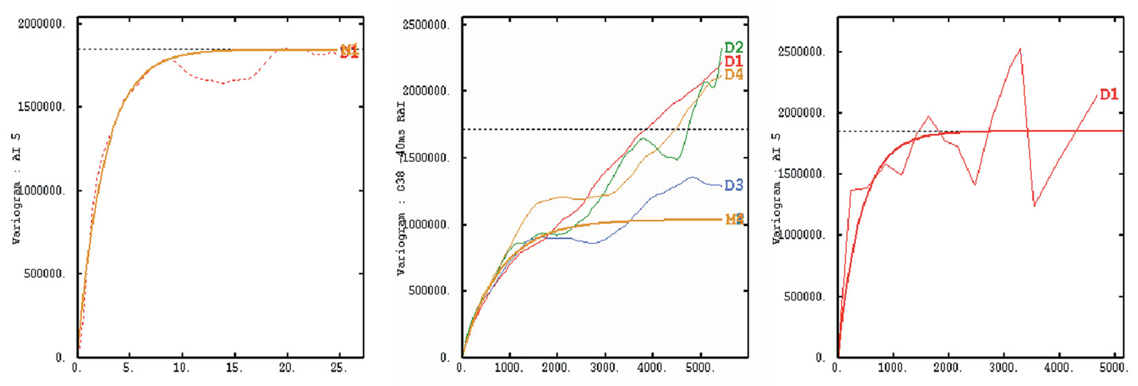
An example using the Stratton 3D dataset (Levey et al, 1994) is shown here. An initial model has been constructed in 3D in the time domain using 14 wells within the 3D cube. Variograms are calculated to provide the geostatistical inputs to the model. Vertical variograms are computed directly from the well logs. The ranges for the horizontal component of the variograms are estimated from horizon slices through a coloured inversion of the seismic volume. Examples of the variograms are shown in Figure 3.

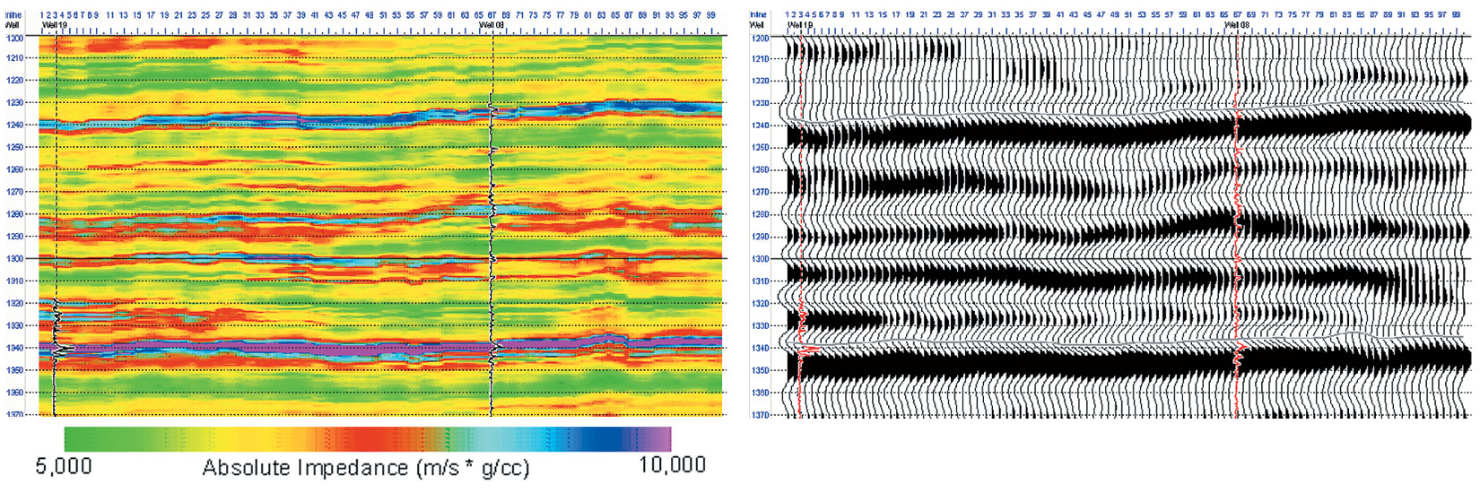
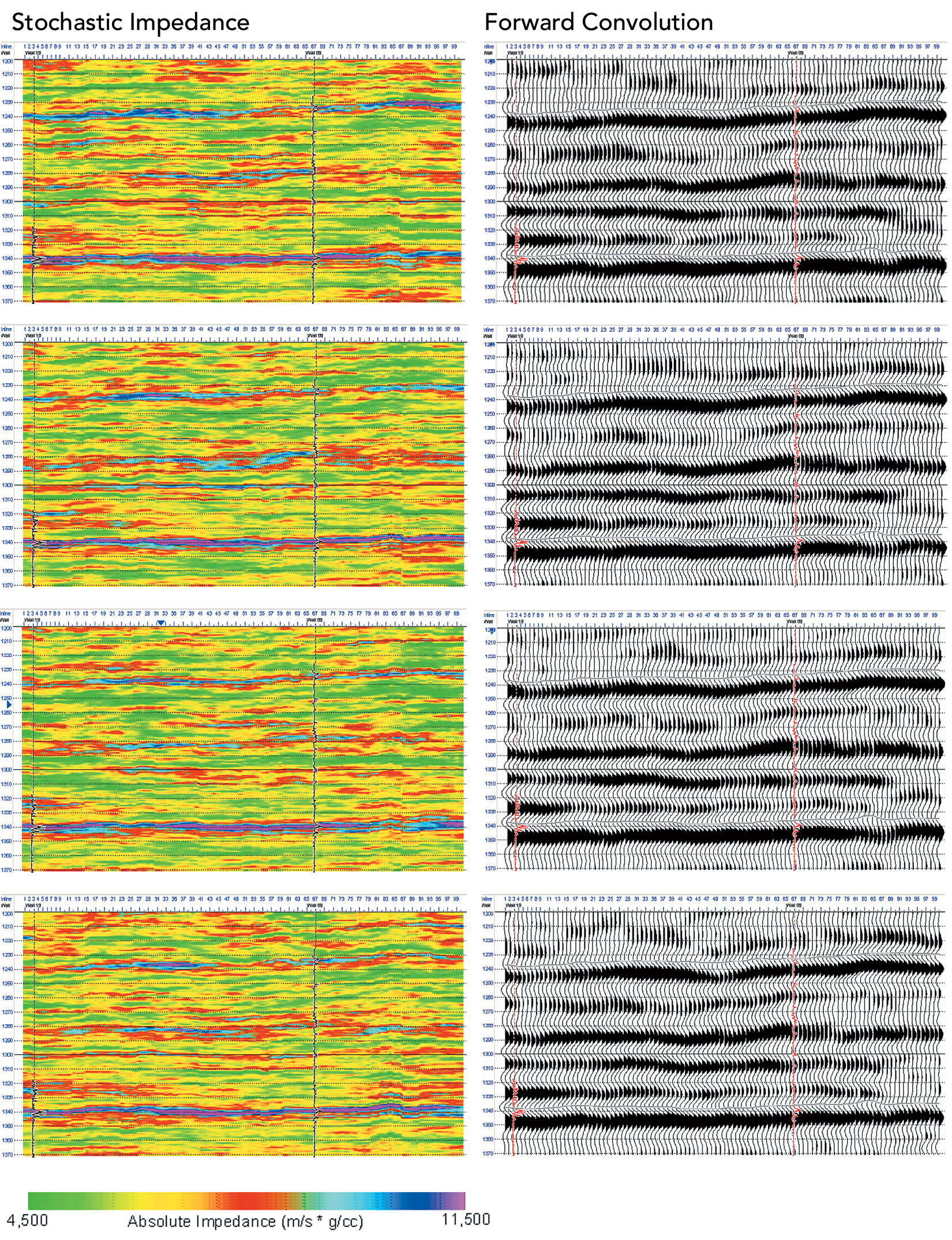
The deterministic inversion result is shown in Figure 4 (with the original seismic section adjacent). Four impedance realisations from the stochastic seismic inversion are shown in Figure 5 together with the forward convolution to a synthetic seismic section adjacent to each. Comparison of the synthetic sections with the real seismic in Figure 4 confirms each realisation is conditional to the seismic.

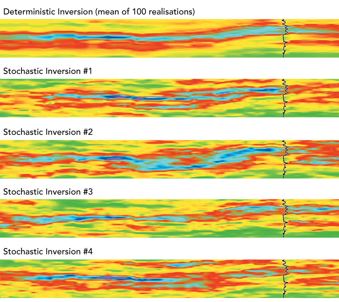
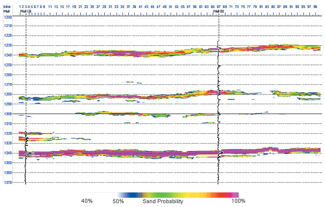
Comparison between the impedance realisations shows how significant non-uniqueness is in seismic inversion. Figure 6 shows a detail comparing the sand located near the mid time (1280 ms) shown in Figures 4 and 5. The top panel in Figure 6 shows the average of 100 realisations (equivalent to the deterministic inversion) and below are the four example realisations. Note how the sand appears continuous and connected to the well in the top panel (sands are higher impedance in blue), but the subsequent realisations show how non-unique the inversion is, with the first showing three stacked sands, the second a thick, connected sand, the third a thin, disconnected sand and the last shows two thinner stacked sands not connected to the well. The continuity and thickness variations between just these four realisations are highly significant and the non-uniqueness may be surprising.

Using an impedance cutoff to approximately indicate clean sands, the net sand in the entire impedance cube has been computed from the deterministic inversion and for each of 100 stochastic impedance realisations. The deterministic inversion gives a net sand of 8.5 % whereas the impedance realisations range from 11.6 to 15.5 % with a mean value of 13.5 % net sand.

The wells show an average net sand of 13.2 %. The cumulative distribution function of net sand is shown in Figure 7, with the averages obtained from the wells and the deterministic inversion also indicated.

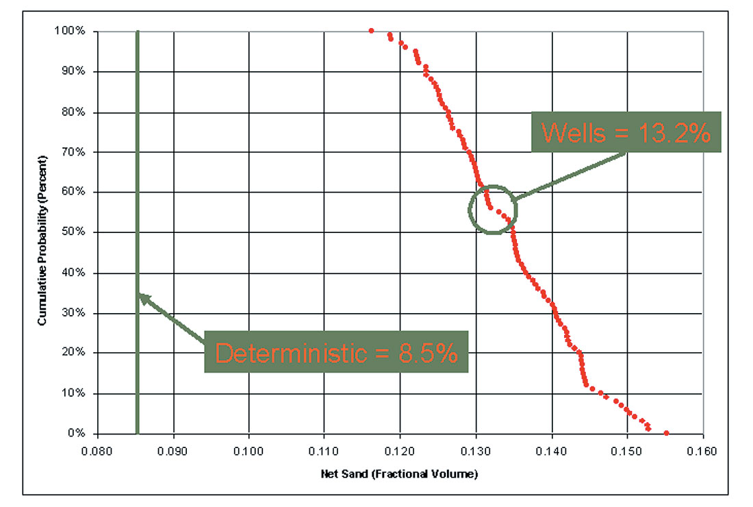
The significant under-prediction of net sand from deterministic inversion is expected from geostatistical theory. Deterministic inversion schemes are unable to reproduce the full range of impedance as their output is optimal and therefore smoother than the impedance observed at the wells. If we truncate the distribution and integrate samples above a cutoff we will find too few samples and hence systematically underestimate net sand volumes. The stochastic inversions, whilst uncertain and non-unique, do reproduce the impedance distribution and therefore there is no bias when we apply the cutoff. By looking at many realisations, the uncertainty in net sand variation is quantified, as shown by the distribution curve of Figure 7.

We can make further predictive use of the impedance realisations. For each stochastic inversion realisation we check if each time sample is classified as clean sand. By counting the proportion of realisations which show the sample as clean sand, we obtain the probability of sand at this sample. The resulting cube is sometimes referred to as an iso-probability cube and the result calculated for this data is shown in Figure 8. The colour table is arranged to show a P50 (chance of 50%) or better of being clean sand. Using a voxel system to pick the P50 envelope of the sand a round 1280 ms from this volume we can then compute the P50 isochron and hence P50 thickness of the sand. As a comparison this has also been done for the deterministic inversion and the two sand thickness maps are compared in Figure 9. The deterministic net sand map has less sand predicted and is generally thinner. The channel in the top left (NW) corner of the P50 stochastic net sand map is nicely defined but not evident at all in the deterministic net sand map.

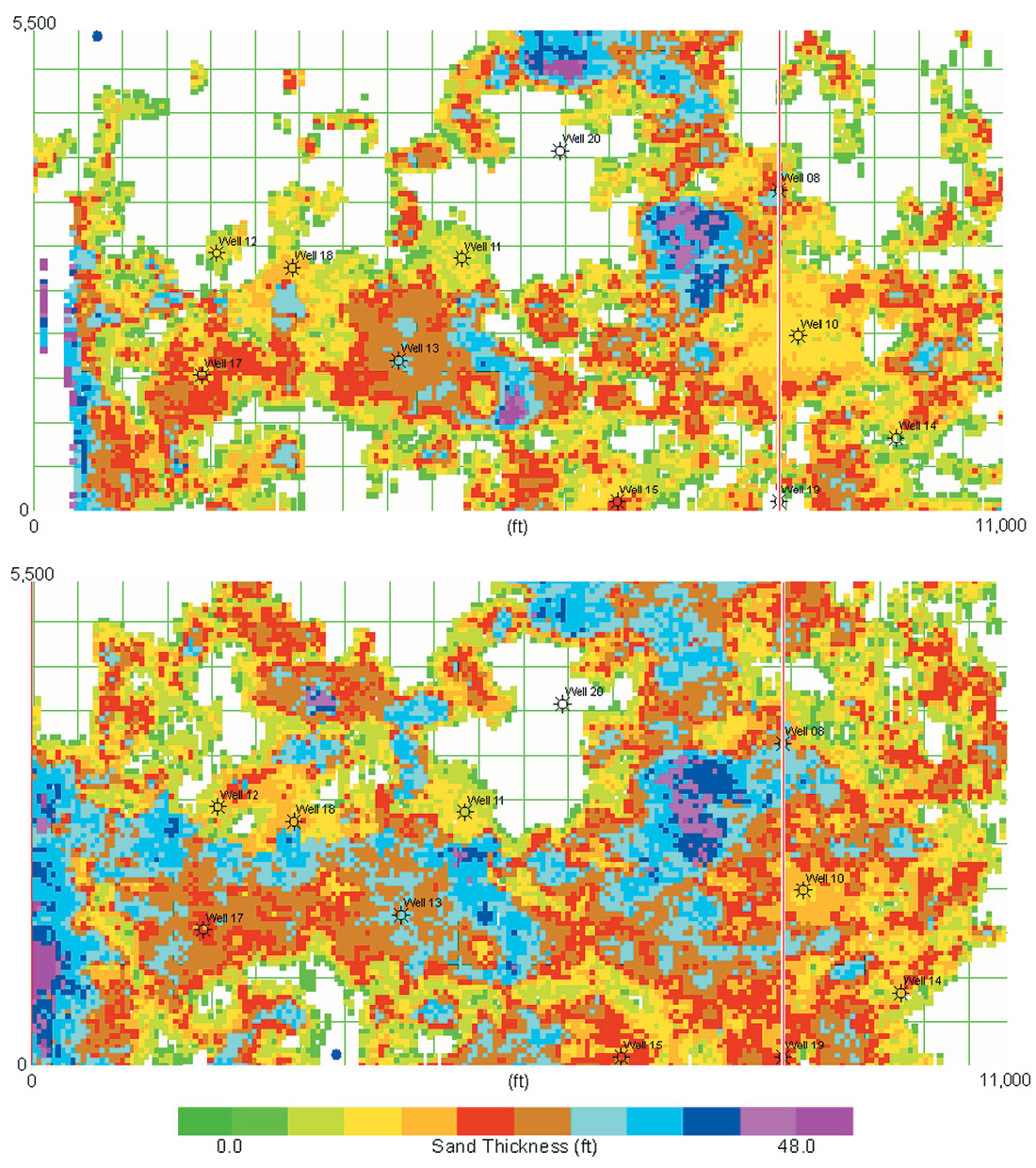
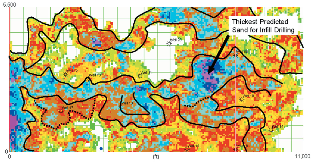
Figure 10 shows a possible interpretation of the P50 net sand map derived from the stochastic inversion realisations. The channel at the top is clearly defined, together with the thick depositional trend across the centre of the area. A possible splay is interpreted around Well-17 and an abandoned meander (oxbow) adjacent to Well-13.