Interpreting Microseismic Data from Hydraulic Fracturing: Understanding Subsurface Deformation Through Numerical Modeling

This article is a summary of the results presented in the PhD Thesis written by Boroumand (2016). The developments made in the research sought to find an answer to the question “why and how did the hydraulic fracture(s) grow in a particular direction?” It makes specific use of microseismic observations to calibrate measured hydraulic fracture geometries in time and space to modeled dimensions so that a geomechanical interpretation of the deformation process could be made. First, section 1.1 looks at the energy considerations associated with hydraulic fracturing with emphasis on correcting for radiated seismic energy. While section 1.2 presents a novel approach in which microseismic locations are incorporated into an energy-based numerical model. Finally, section 1.3 describes how an iteratively coupled three dimensional (3D) stress and flow numerical scheme can be used to explain the microseismic observations and deformation behavior.

Introduction

Microseismic events, symptomatic of induced hydraulic fractures, are used to characterize and image fracture evolution in time and space. Passive seismic monitoring systems are deployed in boreholes and/or on surface to record the events that occur in the destabilized regions surrounding the hydraulic fracture(s). There have been several examples of geomechanical simulations and numerical illustrations tying microseismic event distributions to hydraulic fracturing (Guest and Settari., 2010; Boroumand and Eaton, 2015). Fracture models are typically used to design treatment programs prior to executing the job in the field. But, a post-fracture interpretation which incorporates microseismic data can yield valuable insights that could be used to improve and optimize future treatment design. When microseismic observations, located with enough accuracy, are used to constrain a geomechanical model, one can take full advantage of their interpretive potential. The purpose of numerical simulations is to run a number of deformation scenarios prior to conducting a treatment so that: 1) the ideal treatment can be designed that maximizes deformation, but limits fluid loss and unnecessary out of zone growth and 2) treatment plans can be revised to limit the potential for induced earthquakes. The three sections presented in this article explain the tools developed, analysis and evaluation approach that can be used for value added microseismic interpretation.

1.1 Microseismic energy

There are several energy considerations associated with the mechanics of hydraulic fracturing (Advani et al., 1990). A summary of a few of the energies is provided in Boroumand and Eaton (2012) and expressed as a percentage of the total injected energy (E_I). Aside from energy loss due to fluid dissipation, friction, hydrostatic and energy absorbed by the fracture fluid, the results showed that the fracture energy (E_F) contributes the most to the total useful output energy and that the radiated seismic energy (E_S), even after a b value energy correction, was less than 1%. Fracture energy is the energy required to open the fracture and is associated with the effective bottomhole pressure and E_S is the sum of all individual microseismic energies.

For hydraulic fracturing, microseismic locations have brought new capabilities for understanding subsurface deformation. Their energies are generally small and are not a significant part of the dissipated energy (Maxwell, 2011). If a fault is activated during a treatment (Maxwell et al., 2008) or seismic events are induced, then ES can increase significantly.

Figure 1 presents values for E_S, from a single fracture treatment, before (i.e. observed) and after (i.e. predicted) the b value energy correction for missing data. The method uses Kanamori’s (1977) formula for earthquake energy, modified from the Gutenberg-Richter (G-R) magnitude-energy relation, Gutenberg and Richter’s (1954) frequency-magnitude distribution (FMD) relation and Aki’s (1965) maximum-likelihood (MLE) method to make the correction. The b value is the slope of the line that forms on the FMD plot (see figure 1a).

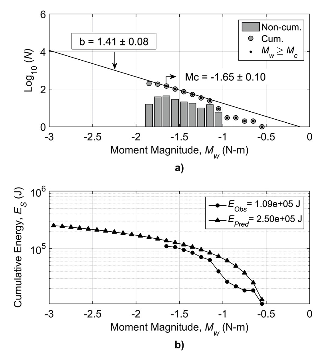
In conclusion, given that ES < 1%, the microseismic events are largely associated with and closely related to the hydraulic fracture deformation process rather than fault activation or induced seismic activity. Moreover, energy analysis can be used as an interpretative tool to determine changes in microseismic activity across a field, well and completion stages.

1.2 Mechanics of hydraulic fracturing

This section presents a novel approach that explains hydraulic fracture behavior, from an energy-balance perspective, using the spatial-temporal evolution of microseismicity to constrain and validate the model.

The energy-based numerical algorithm is developed to propagate a planar hydraulic fracture and match its modeled dimensions to those inferred from the microseismic map. This is primarily done by making adjustments to the input parameters programmed into the model. The code written to produce the simulations was based on previously published methods by Advani et al. (1990), Lee et al. (1991) and Moon (1992).

The partial differential non-linear equations that govern the numerical model are based on the Lagrangian formula detailed in the work presented by Advani et al. (1990). The algorithm that simulated a fracture, contained problem-specific coordinates corresponding to the major (i.e. half-length) and minor semi-axes (i.e. half-height and half-width) of an ellipsoid. The energy balance formula contained the term U_p, which is the energy required to open the fracture using an effective pressure, the energy corresponding to the crack opening width is U_s, the Griffith fracture surface energy for crack propagation is U_f and the fluid dissipation energy rate term, including leak-off effects, is Ḋ.

Two parameters were adjusted to calibrate the fracture model to microseismic data; fracture length was fitted by altering an empirical parameter, fracture toughness (e.g. figure 2b), and observed upward growth was fitted by adjusting stress barrier contrasts (e.g. figure 2c). In the case of a symmetric model with equivalent stress and material properties above and below the fracture, an increase in fracture toughness resulted in a corresponding increase in modeled net pressure and fracture width profile. In the case of a model with different stress states in the layers above and below the injection level, fracture height growth is enhanced in the layer with lower in situ stress. In both cases, net work is minimized in response to trade-offs between the creation of new fracture surface area and fracture volume.

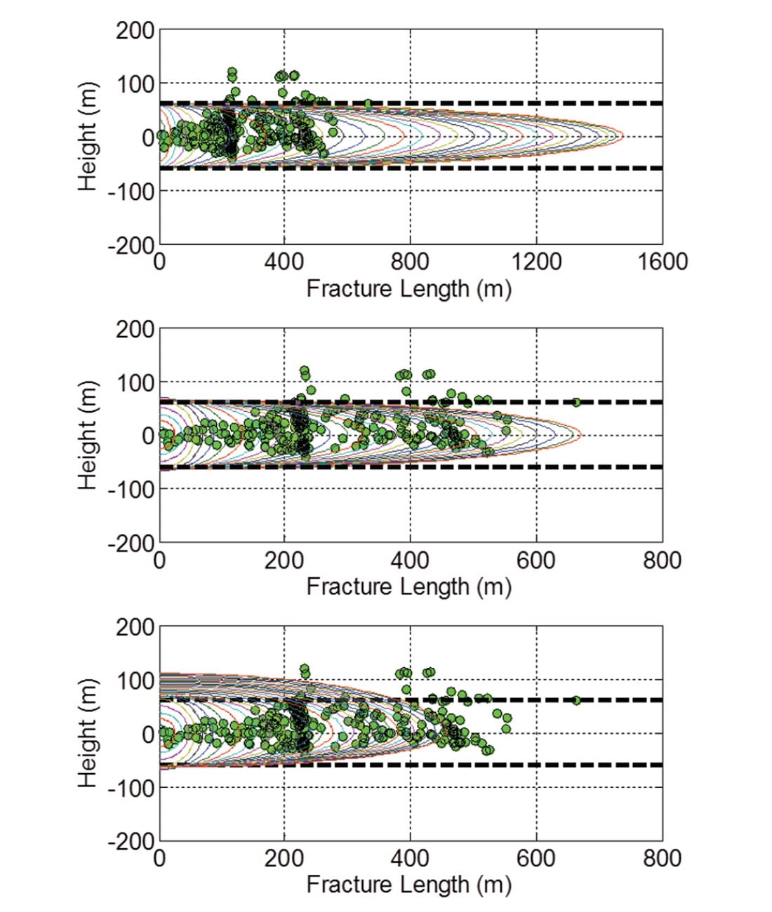
Figure 2a shows the simulation results using default input parameters, figures 2b and 2c show a match between the length and height of the simulated fracture geometry to those inferred by the microseismic map respectively.

A complete version of this work was published by Boroumand and Eaton (2015) and provides a detailed analysis on the effects of parameter selection on fracture propagation. The results showed that a match between real and model data could be achieved with optimum parameter selection. By understanding the fracture behavior and the influencing variables, decisions regarding fracture design, stage spacing, well spacing, and pad positioning can be optimized.

1.3 Fluid and geomechanics numerical simulation

This section shows the advanced analysis that can be done through an iteratively coupled 3D stress and flow numerical algorithm. The deformed regions in the stress-strain model, caused by fluid diffusion and displaced rock from fracture propagation, are where microseismic activity develops. Visualization of the displacement field, fluid diffusion, compression and shear zones with the microseismic observations can lead to improved interpretability of subsurface deformation.

The volume coupling scheme of Settari and Mourits (1998) was used to balance the pressure distribution between the 3D diffusion and stress distribution in the geomechanical model developed for this section. This interaction is based on the change of porosity using Biot’s formula (Biot, 1941; Detournay and Cheng, 1993). In brief, the fluid flow follows the diffusion model from Wangen (2011; 2013), while the geomechanical model is built using Hooke’s Law, applying Newton’s Second Law to consider volume that forms the Navier displacement equation.

The numerical simulation using the coupled fluid and geomechanics code containing a fracture propagation criteria was run to evaluate the effects of input properties on fracture propagation. The single stage tested had microseismic data which was matched in time and space with the simulation results. The duration and all equivalent inputs to the model were scaled to fit the field data and yield faster computation time.

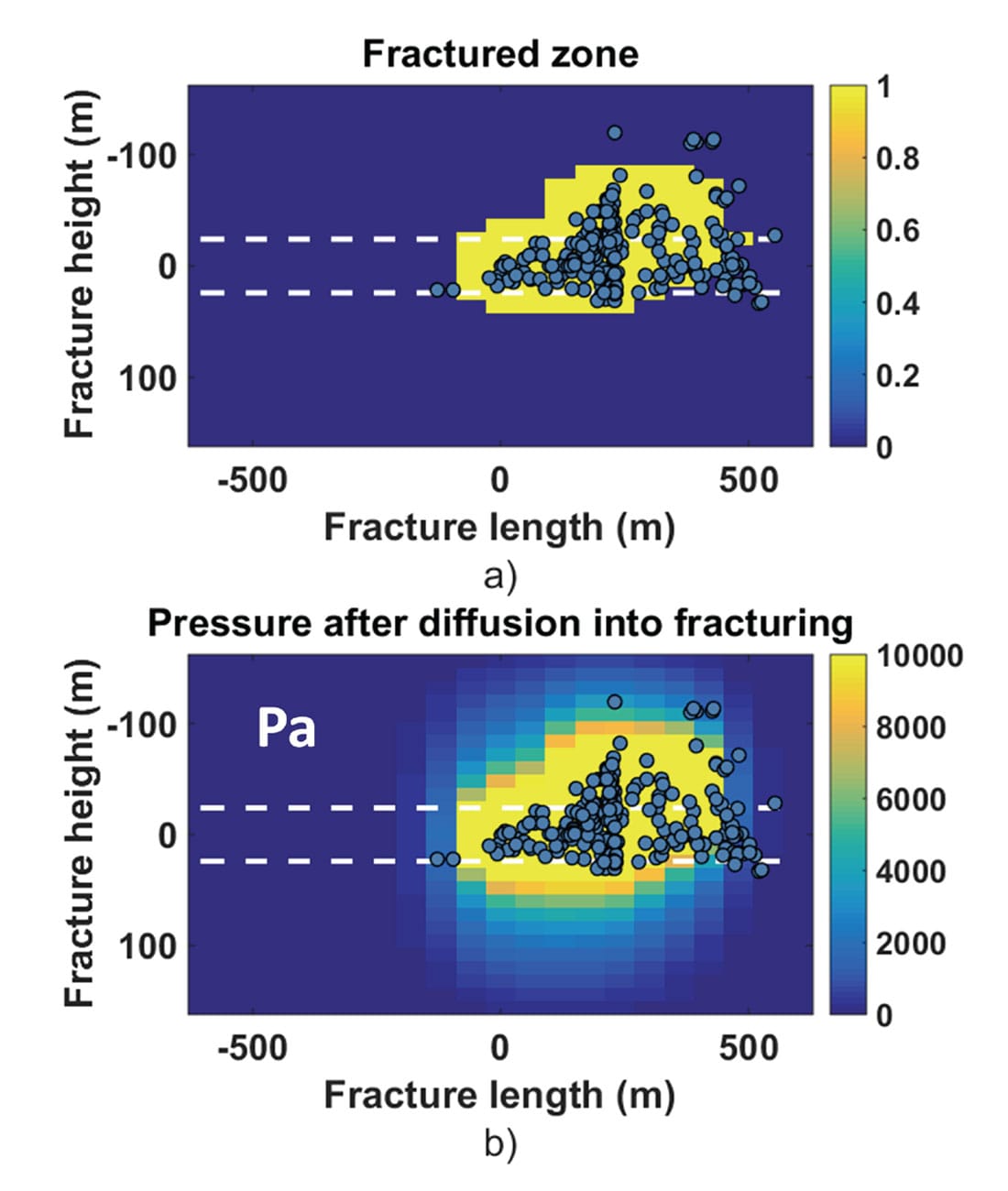
Figure 3 shows the final time step of the propagated fracture overlain with the microseismic event locations. The white fracture zones (figure 3b) showing high pressure, correspond to the fractured region (figure 3a) where the pressure is expected to be the highest. Note, microseisms are plotted on top of the white zone, but are not actually located inside the fracture; they occur outside of the hydraulic fracture on either side of the fracture surface, but are plotted to show the correlation between the microseismic population and the location of the deformed regions. The light grey region surrounding the edges of the 2D fracture, have elevated pressure (compared to regions beyond the fracture itself) due to fluid diffusion. These areas are the fracture tips corresponding to high shear stress and where microseisms are known to occur.

The stress barrier contrast for the upper layer was reduced compared to the target zone to match the upward growth observed from the microseismic events. The stress barrier for the lower layer was increased to prevent downward growth. The microseismic observations did not show downward growth, so it seemed fitting to assign a barrier for this zone. Adjustments to the stress values impacting height growth enhanced upward growth but suppressed downward growth.

Adjustments made to the stress and fracture toughness properties showed that they have a significant impact on the spatial and temporal evolution of the hydraulic fracture. Furthermore, by means of parameter adjustments using microseismicity as a constraint, an interpretation explaining the timing of the deformation and its location was possible.

Conclusions

Since its inception, microseismic mapping has brought new capabilities in the way of characterizing fracture propagation. A few of these advancements, mainly those developed and investigated in this research, are summarized below.

Section 1.1 showed that although a b value correction was needed to account for missing data, the results demonstrated that radiated high-frequency from radiated seismic energy represent a very small component of the overall energy in the hydraulic fracturing system. If and when this value exceeds the fracture energy, then it could imply that a fault is activated or seismic activity has been induced.

Section 1.2 showed that through an energy based numerical simulation, accounting for the various physical deformations, parameter selection tied to microseismic observations can yield a better understanding of subsurface processes. By understanding the fracture behavior and the influencing variables, decisions regarding fracture design, stage spacing, well spacing, and pad positioning can be optimized.

Section 1.3 showed that a combined analysis of fluid flow and stress/strain interactions, via a coupled numerical algorithm while calibrating to microseismic event locations, permits a deeper understanding of the subsurface processes.

When one takes full advantage of microseismic observations by incorporating them into numerical simulations, the mystery behind why fractures grow the way they do can be uncovered. This knowledge and understanding leads to improved well completions, fracture designs and improved field development.

Acknowledgements

Sponsors of the Microseismic Industry Consortium are thanked for their support of this work. We are particularly grateful for support from the Natural Sciences and Engineering Research Council of Canada (NSERC) and Chevron for their support of an Industrial Research Chair in Microseismic System Dynamics at the University of Calgary. We would also like to thank Nexen Energy ULC, Spectris plc (ESG Solutions) for providing the data to conduct this research. We are also grateful for the many valuable discussions had with Hassan Khaniani, Norm Warpinski, Tony Settari and the various students and staff within the UofC and UofA group over the years.