Interpretation of Aeromagnetic Data

Introduction

The previous three articles of this series on Potential Field (PF) Geophysics dealt with recent technical improvements in magnetics and gravity instrumentation as well as with critical components concerning data acquisition and PF project management. This article focuses on processing and interpretation of aeromagnetic data. Key aspects of each of these processes will be illustrated using examples from a High Resolution AeroMagnetic (HRAM) survey over an area near the Sierra Reef in NE British Columbia.

Why is there suddenly so much interest in aeromagnetics in Western Canada? The simple answer is that now it is possible to map intra-sedimentary faults and fractures which are magnetized, whereas before the magnetics was used primarily to decipher basement tectonics. The interpretive result is a structural grain map which complements seismic interpretations, covers a much larger area, and the total cost is very modest by seismic standards.

Processing

1. In Field Quality Control (QC)

Proper data processing begins in the field. In-field processing is a crucial component of quality control by the contractor. This QC will provide an early indication of acquisition problems and allow the crew to remedy deficiencies before proceeding further with the survey. The results from field processing also allow the client to have effective, independent on site quality control.

2. Cultural Editing

Until the last few years, most aeromagnetic data have been acquired at relatively large distances above the ground and with magnetometers of less sensitivity than are now used. Consequently, cultural interference was less a concern. Today, HRAM surveys are flown at low ground clearances (sometimes less than 100 m). Consequently cultural noise has become a serious problem, although its deleterious effects are not yet universally recognized.

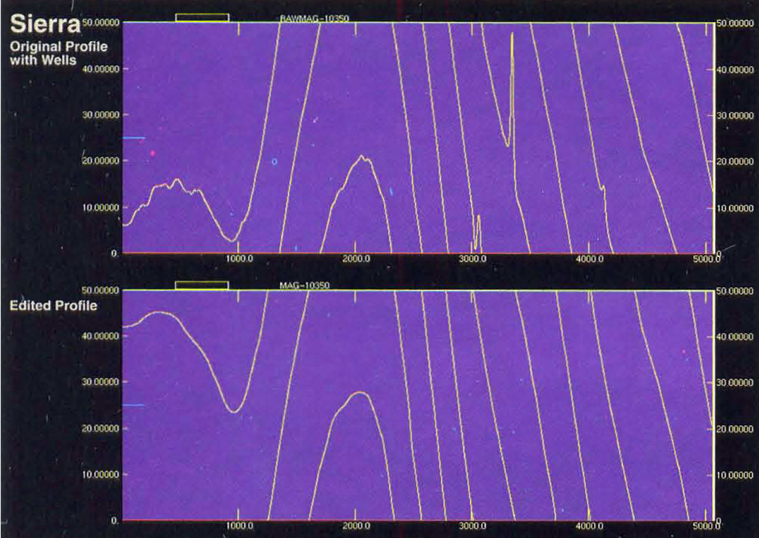
The data sets delivered by acquisition contractors are carefully levelled to remove any misties at line crossings, and no editing of cultural features is normally done. Cultural features such as wells, pipe lines, bridges, processing plants, etc. generate sharp magnetic anomalies. A typical anomaly caused by a cased well is a spike of 8-20 nT if the plane passes directly over the well, or it may be a much more subtle peak of < 1 nT if the flight path is 100 m away from the wellhead (Fig. 1, upper panel). The detrimental effects of cultural noise become very visible in residual and derivative data products where they obscure much of the subtle signal. Furthermore, because cultural noise is spike-like, any digital filtering of the data set will cause ringing effects, enlarging the size of the anomaly and sometimes showing up again in aliased harmonics. The solution is to edit the profiles as the first step in interpretive processing (Fig. 1, lower panel).

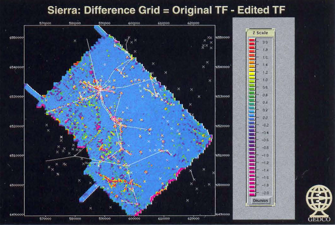
Efficient editing of cultural anomalies requires special software, reliable knowledge of cultural surface sources, good in-flight video and last, but not least, a competent geophysicist who can remove the cultural interference effect without changing the subsurface geological response. In most cases, the more dominant cultural anomalies are removed quite easily, while more difficult anomalies, due to some pipe lines and power lines traversed at acute angles, can be very tricky to filter from the data. We estimate that perhaps 90% of the cultural interference can be removed from a typical data set from Western Canada. As the density of cultural effects increases, it becomes harder to remove just the culture without also affecting the higher frequency components of the geological signal. Figure 2 shows the difference between unedited and edited data for the Sierra survey, calculated by subtracting the edited data grid from the unedited data grid.

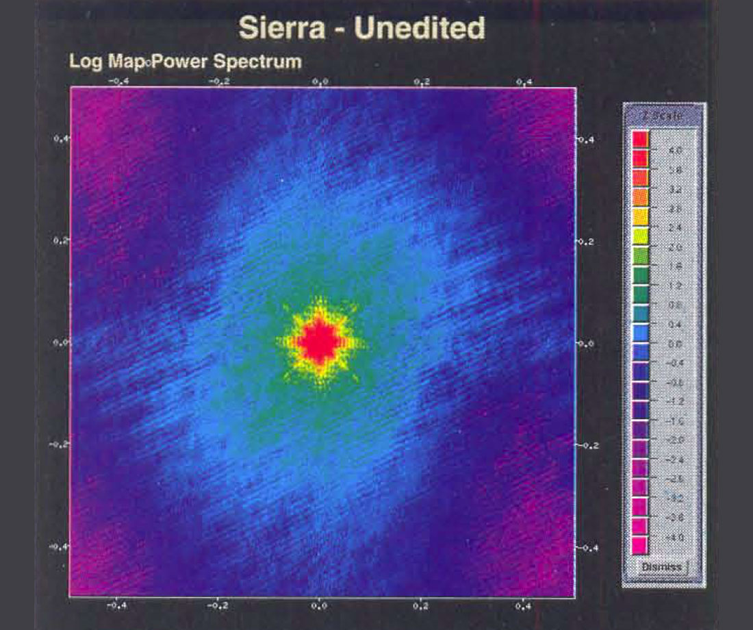
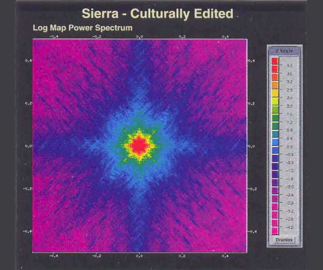
The improvement in signal/noise ratios before and after editing on this particular data set is illustrated in the respective map spectra. Figure 3 shows the power spectrum of the unedited data, with low frequencies and high power at the centre, grading out to higher frequencies and low power levels at greater radial distances. The survey lines were oriented NE/SW and the control lines NW/SE, giving rise to the NW/SE and NE/SW lines of coherent noise seen near the centre in the yellow part of the spectral display. The somewhat broader EIW and N/S lines of coherent noise are caused by the griding, which was oriented N/S and EIW. Less distinct lines of coherent noise can be seen further from the centre in the green and blue colours, oriented at approximately 0300 and 0600. The repeated nature of these lineations indicates ringing from the application of filters. In most cases we can identify the source of such coherent spectral energy, but in this case we do not understand its source. However, after cultural editing, the map spectrum of the edited data (Figure 4), displayed with the same colour scale, does not display the ringing noise lines. The power level at higher frequencies is lower (more violet colour), indicating higher signal to noise ratio. The effect of the flight line noise and griding noise is now evident throughout the frequency range displayed.

Editing even a small number of profile effects the statistics of line misties. It is therefore mandatory to bi-directionally re-level the data to produce a final processed data set.

3. Griding, Filtering and Mapping

Applying a low amplitude Wiener filter (0.1 - 0.25 nT) to the re-levelled profile data is a prudent first step to remove residual low amplitude noise. We also apply such a filter after griding to suppress grid noise.

The choice of grid cell size is very important. If one is using a standard rectangular griding algorithm then we recommend that the grid cell size be no smaller than a third of the traverse line spacing in order to avoid excessive grid noise in the filtered products. A problem concerning the grid cell size may occur for surveys where wider line spacing is quite sufficient for geophysical reasons and where an image type display of the results is desired. A larger grid cell size is usually not suited for higher resolution image displays. Regriding and anti-alias filters are a valid way around this dilemma, although the results may lack the resolution desired.

The next step is the application of a Reduction to the Pole (RTP) filter. This filter applies a latitude dependent phase shift to centre an anomaly peak over its source. (Note: Such a filter is usually standard for Canadian data, but at the low magnetic latitudes encountered in many international projects, a Reduction to Equator (RTE) may cause less amplification of noise than the RTP filter. Low latitude survey designs must consider these additional complications.)

Filtering allows one to quickly analyse large data sets. Because the wavelength of the magnetic anomaly is strongly dependent on the depth of the source, band pass filters can be used qualitatively to separate deeper sources from shallow sources. Vertical derivative filters amplify the high frequency components of the data, and horizontal derivative filters produce an "edge" map where the high data values are centred over the edges of the magnetic sources (e.g. to highlight faulting relationships.) More precisely, tuned spectral filters can optimize the depth resolution of the result, but they are somewhat more complicated in that they must be designed from spectral analysis of the data. Strike filters can be used in special situations to suppress or enhance trends.

The cover shows an example of a band pass filter designed to highlight anomalies arising from the upper basement and the lower sedimentary section. Because the Precambrian surface is at about 2500 m depth (sub-surface) in this area, we can expect that anomalies caused by sources near the Precambrian surface to have dominant wavelengths of about 5000 m. Applying a 1.5 - 7 k:m band pass filter to the edited total field data (cover, upper image) suppresses the long wavelength anomalies from the lower crust and produces a dramatically different perspective (cover, lower image). The upper image shows the total intensity aeromagnetic map over the area around the Sierra Reef, NE British Columbia, after editing. Red and yellow colours are highs; blue and magenta colours are lows. The lower image shows a band pass (1.5 - 7 km wavelength) of the same data in shaded relief format. Illumination is from the NE; red and yellow colours are highs; green and blue colours are lows. Structural contours on mid-Devonian carbonate, taken from B.C. Government map, are shown. Several geological features are highlighted. Note that where the structural contours narrow at the upper end of the Junior Embayment is related to a basement fault which offsets the magnetic anomalies. Note also the Yoyo Magnetic High, which runs south from the Yoyo Reef. This correlates with a poorly defined basement high on which the Yoyo Reef apparently nucleated. The lower image shows a band pass (1.5 - 7 km wavelength) of the same data in shaded relief format. Illumination is from the NE; red and yellow colours are highs; green and blue colours are lows. Figure 5 shows a higher frequency band pass (0 - 4 km) of the same area. The filter was designed to minimize the effects of basement and show the intra-sedimentary magnetic fabric.

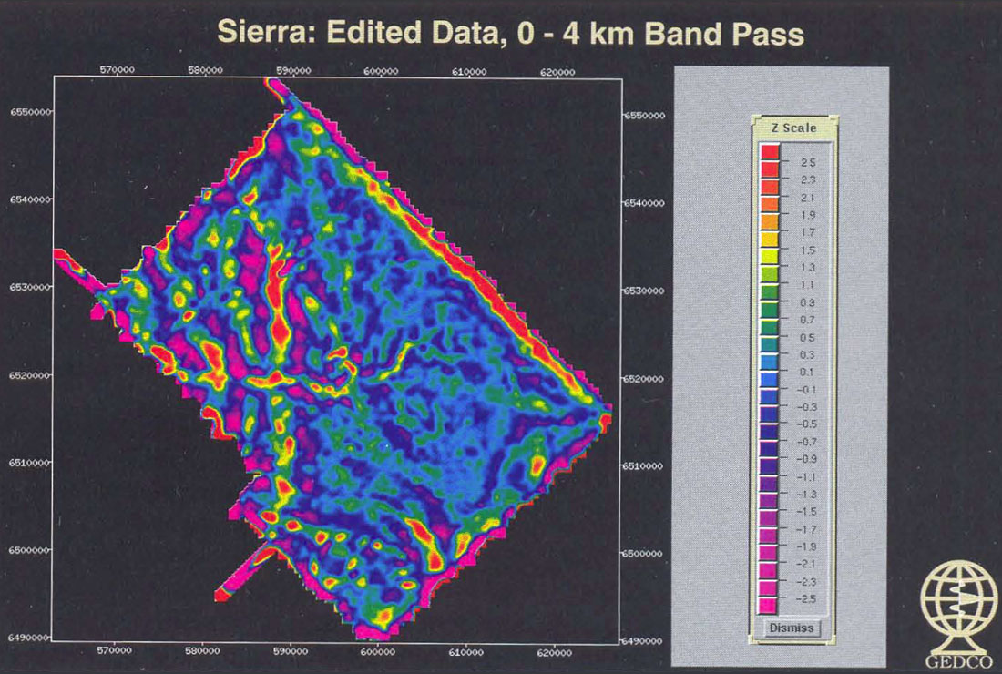
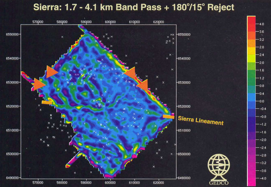
Figure 6 is a combination of filters which were designed (by empirical experimentation) to highlight an E/W striking feature which we have named the Sierra lineament. In this case, a strike filter was used to suppress the strong north/south Yoyo Magnetic High.

Display formats certainly have changed over the years with ever more visualization software available. The display format can be simple contours, colour contours, shaded relief or colour shaded relief. The final display depends on the frequency content of the data, the features one is trying to highlight, and what can be done to display the results in the most telling manner. It is very important that an appropriate choice of scale is made and that the map is annotated sufficiently for the user to be able easily to cross-reference the results with other information.

Depth Interpretation of Profiles

It is somewhat strange that often less emphasis is placed on interpreting the profile data for depth information than in previous years, when data accuracy was lower. Grid products provide an excellent qualitative perspective; but, except for some 3-D inversion attempts, it is still necessary to interpret the profiles to extract quantitative depth information. Depth analysis of the profiles is time consuming and requires appropriate software, but the results are definitely worth it as they provide a reasonably precise estimate of the depth distribution of a magnetic source rather than simply 'seeing' a lineament on a map.

We recommend using a combination of depth estimation techniques in order to obtain the best results. Some of the methods respond better than others to certain amplitude/frequency combinations, profile length and frequency content. Well documented methods such as Werner and 2D Euler are our mainstays. Somewhat less known but useful supplementary techniques are the spectral and gradient analysis and the Phillips method, as well as the 'old' manual methods, such as Peters slope technique, and a series of mostly Russian manual estimation approaches implemented interactively on screen. (Another digital depth estimation technique is 3D Euler, applied to gridded data, and used primarily in the mining industry.)

The Werner and Euler techniques calculate the position of point sources which could cause the anomalies for various data windows along the profile. Both techniques calculate a large number of possible sources. Clustering techniques are used to accept only those sources which are tightly grouped. If several solutions are tightly grouped in space, they are more likely to be valid. The software plots these clusters (circles and crosses on Figure 7) in a depth section along with the profile (and its gradient or derivative) above. Even after clustering, there is still a plethora of solutions plotted. At this point an experienced geophysicist must assign some geological meaning to them.

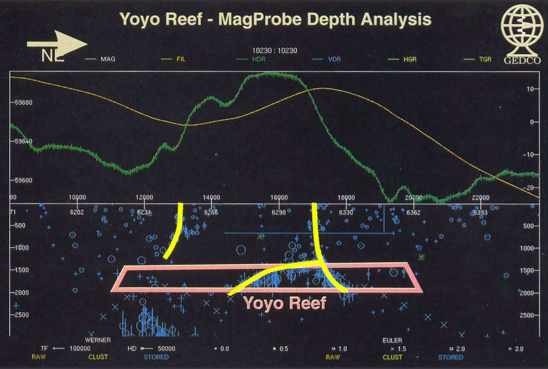
Figure 7 shows the results of depth interpretation on a profile which crosses the Yoyo Reef. (This particular profile was relatively uncontaminated by cultural noise due to the producing wells and the gas plant.) The depth estimates are plotted as a depth section, with the x-dimension being distance (m) along profile and the z-dimension being subsea depth (m). The position of the Yoyo Reef has been drawn in schematically for reference. Note the grouping of depth estimates highlighted by the yellow lines. The line above the word reef is interpreted as a magnetized east-dipping, listric fault plane which appears to pass through the reef. This intra-sedimentary fault or fracture is spatially associated with the eastern side of the basement ridge marked by the Yoyo Magnetic High. A less well defined fault or fracture is interpreted on the SW side of the reef, and this is associated with the west side of the same basement ridge.

If the results of the depth interpretation are plotted at the scale of the filtered maps, then the positions of these fault interpretations can be correlated in map format. The result is a structural grain map which in many ways resembles a LANDSAT image interpretation, but one can colour code the results to indicate which faults are intra-sedimentary and which arise from the basement.

Modelling

Magnetic modelling can be very helpful for determining basement structure when there is significant relief and basement composition is relatively uncomplicated in terms of susceptibility variations. To date, magnetic modelling of intra-sedimentary anomalies has not been widely used. Whenever possible, models should incorporate other constraints, particularly well control when available, as well as seismic and gravity data. Several excellent modelling modules are available, and some software can now interactively display the seismic control with the potential field model.

Conclusions

High resolution aeromagnetic surveys are now producing new perspectives of sedimentary structures. The increase in resolution has been achieved, in large part, because of the increased navigational accuracy provided by the global positioning satellite (GPS) system, operated in differential mode. Better magnetometers and drape flying close to the ground are used to sample the higher frequencies, and the computer power of work stations is used to analyse the data rapidly and to visualize it in ways that simply were not feasible a few years ago. The results are new and often startling. As with any new technique which opens up new vistas of interpretation, interpretive methods are evolving rapidly and novel ways to apply the new information gained are close behind.

Acknowledgements

The Sierra aeromagnetic survey was acquired in 1994 by Questor Surveys Inc., a subsidiary of World Geoscience Corporation. The data are available from Petroseis90 Inc. The area shown is about 40 x 55 km. The authors thank Debi Walker for producing the figures for this paper and Brian Henry for a valuable critique of our original draft.