Interbed Multiple Prediction on Land: Which Technology, and Which Domain?

Prediction and removal of internal or interbed multiples is an increasingly high priority problem in seismic data analysis. One reason for the growth of its role and importance comes from the increased sensitivity with which primary amplitudes in quantitative interpretation are now analyzed. But the importance of accurate and robust prediction of internal multiples may now be on the verge of an even greater upward jump, as full waveform methods come online.

This is counterintuitive at first, because the philosophy of full waveform methods (e.g., full waveform inversion, or FWI) is to treat the entire wave field at once, as a single, unified entity, rather than as a collection of event types (e.g., surface waves, direct arrivals, primary reflections, multiples). If we think of ourselves as working with one complex, undifferentiated wave field, why might we still need to distinguish between primaries and multiples, or any set of event types?

The behavior of FWI and least-squares algorithms tends to be determined through residuals: differences between measured data and modeled data. Updates in the Earth model (in the case of FWI) are decided based on the residuals, as are criteria for stopping the iterations, and so on. One speaks of expending effort to shrink the residuals, but in a seismic data set, where meaningful amplitude differences between modeled and measured waves can exist over an enormous dynamic range, merely finding that the residuals have shrunk may not be enough to judge the value of an iteration or update. A reduction in residuals could be really good news if it is associated with wave events whose propagation paths include zones of interest, but it could also be close to irrelevant if associated with parts of the Earth that are of less interest. Furthermore, a small reduction in residuals could be “better” than a large reduction in residuals if the former is associated with events that have low amplitudes, and the latter is associated with events with large amplitudes. The importance of a change in the residuals could depend critically on the nature of the event in which the residual is reduced. No matter how full-waveform the processing community becomes in the future, having (at least as auxiliary information) detailed knowledge of what event type occurs in the data at specified time will be a critical technology.

Given these motivations, what kind of internal multiple prediction/ removal technology should we focus on? First, a quick review. Multiples are classified as being either surface-related or interbed, distinguished by their interaction (or lack of interaction) with the free-surface. Surface-related multiples can be eliminated because of their periodic character and deterministic predictability, especially in τ-p domain. Many innovative technologies have been developed to do so, such as predictive deconvolution (Taner, 1980, Treitel et al., 1982), inverse approach using feedback model (Verschuur, 1991), invariant embedding technique (Liu et al., 2000), and inverse data processing (Berkhout and Verschuur 2005, 2006).

Here we focus on the prediction/removal of interbed or internal multiples. In practice, this remains a major challenge – especially on land data – even though considerable progress has been made recently. Kelamis et al. (2002) introduced a boundary-related/layer-related approach to attenuate internal multiples in the post-stack data (CMP domain). Berkhout and Verschuur (2005, 2006) extended inverse data processing to attenuate internal multiples by considering them to be effective surface-related multiples through the boundary-related/ layer-related approach in common-focus-point (CFP) domain. The same algorithm was applied by Luo et al. (2007), through re-datuming the top of the multiple generators and transforming internal multiples to be suppositional surface-related. However, these approaches, while powerful, all require significant subsurface knowledge. Multiple prediction and/or removal without a complete knowledge of the velocity structure will almost certainly be required to identify seismic event types before the application of full waveform processing methods, however, the options to perform multiple prediction and/or removal under such circumstances are limited.

Inverse scattering series internal multiple technology leverages the fact that all internal multiples can be estimated through the correct combination of amplitudes and arrival times of primary reflection subevents which satisfy a certain lower-higher-lower relationship in pseudo-depth (Weglein et al. 1997), with generators sought for in the data, in a stepwise and automatic way. This means the primaries will remain intact and no subsurface information is required.

However, challenges remain in the application of these methods, particularly for land data. Luo et al. (2011) list many of the key problematic features encountered in land data, primarily noise, statics, and coupling, each of which cause trouble for multiple prediction algorithms, including those based on the inverse scattering series. To that list we would also add the increased difficulty of selecting algorithm parameters that avoid the generation of artifacts. The search parameter ε (Coates and Weglein, 1996), which limits the proximity of events combined to predict multiples, is normally a single number that is selected in an ad hoc fashion, often guided by the dominant frequency of the experiment. However, wide distributions of shallow generators and generators near zones of interest can make it very difficult to fix on a suitable single value for ε. The use of unsuitable values can be very damaging: if chosen too large, multiples will fail to be predicted; if chosen too small, artifacts correlated with primaries appear in the prediction panel.

We are pursuing two related ways of mitigating artifacts and increasing the precision of single and multicomponent internal multiple prediction on land. The first is acknowledging that a suitable stationary ε value may be impossible to find, and allowing ε to become a function of output variables. Innanen (2016) describes this in detail. The second is to move the prediction calculation into domains in which stationary ε values are found to have less of a negative impact. This paper focuses on the second of these two approaches.

By analyzing the relationship between pseudo-depth and intercept time, building on the τ-p framework of Coates and Weglein (1996) and Nita and Weglein (2009), Sun and Innanen (2015) have noted that an environment with both a relatively stationary search parameter and limited numerical artifacts is in principle achieved. In this paper, realistic synthetics are used to demonstrate the application of the τ-p version of the algorithm on land data. Well logs from the Hussar experiment (Margrave et al., 2011) were used to create synthetic data. The synthetics are based on an acoustic approximation, however, the geological model is constructed to include realistic, log-derived thin layers, and simultaneously large offsets.

Plane-wave domain formula

In presenting the inverse scattering series internal multiple attenuation algorithm, Araujo et al. (1994) and Weglein et al. (1997) showed that all internal multiples can be predicted by summing over events which satisfy what was referred to as the lower-higher-lower relationship in the pseudo-depth domain. Roughly put, this means that internal multiples can be anticipated by the addition and subtraction of travel times of combinations of triplets of events. However, not every possible combination of triplet is used. Only triplets whose travel times are specifically ordered are included: the events whose travel times are to be added must occur later than events whose travel times are to be subtracted. In the early papers on the subject, there was variation in the domain in which the formula was presented. For instance, Coates and Weglein (1996) discussed it in the plane wave domain:

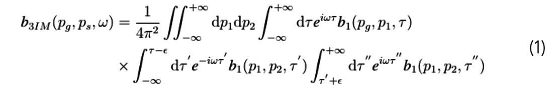
where p_g and p_s are horizontal slowness at source and receiver respectively (these are equal in 1D and 1.5D calculations). The plane-wave formula makes certain kinds of analysis more straightforward (e.g. Nita and Weglein, 2009), and clearly illustrates that the lower-higher-lower rule can be understood equally well in terms of pseudo-depth or vertical travel time. However, recently the plane-wave domain has also been shown to have several practical advantages. Sun and Innanen (2015) point out that in this domain the input is more straightforward to calculate, transform artifacts are naturally suppressed, and, as mentioned above, the optimum ε is more stationary in the horizontal slowness than it is in offset-wavenumber.

The input is the 3D volume calculated by scaling the double τ-p_s-p_g transformed data after sorting into source and receiver gathers, i.e.,

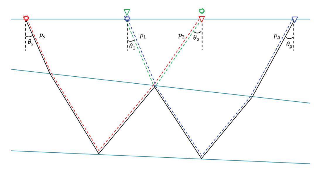
Importantly, here the q_s variable is in units of slowness, and should not to be confused with the vertical wavenumber, which occurs in the form for b₁ in the standard form of the algorithm. Figure 1 illustrates the ray-path relationships between primaries and predicted internal multiples, which can be labeled according to their contributing slowness (p_g, p_s, p₁, and p₂ in equation 1). The quantities p₁ and p₂ represent horizontal slowness at both source and receiver locations within the algorithm. This requires that suites of source and receiver horizontal slowness be equal.

A numerical experiment on CREWES Hussar synthetics

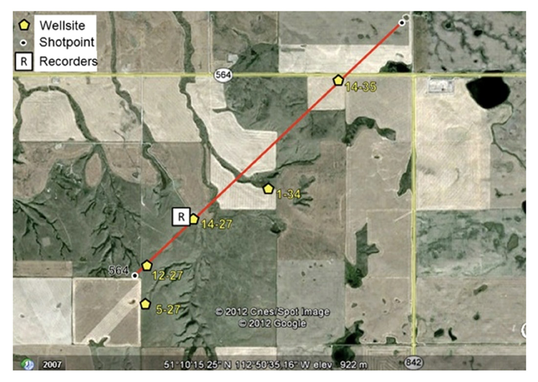
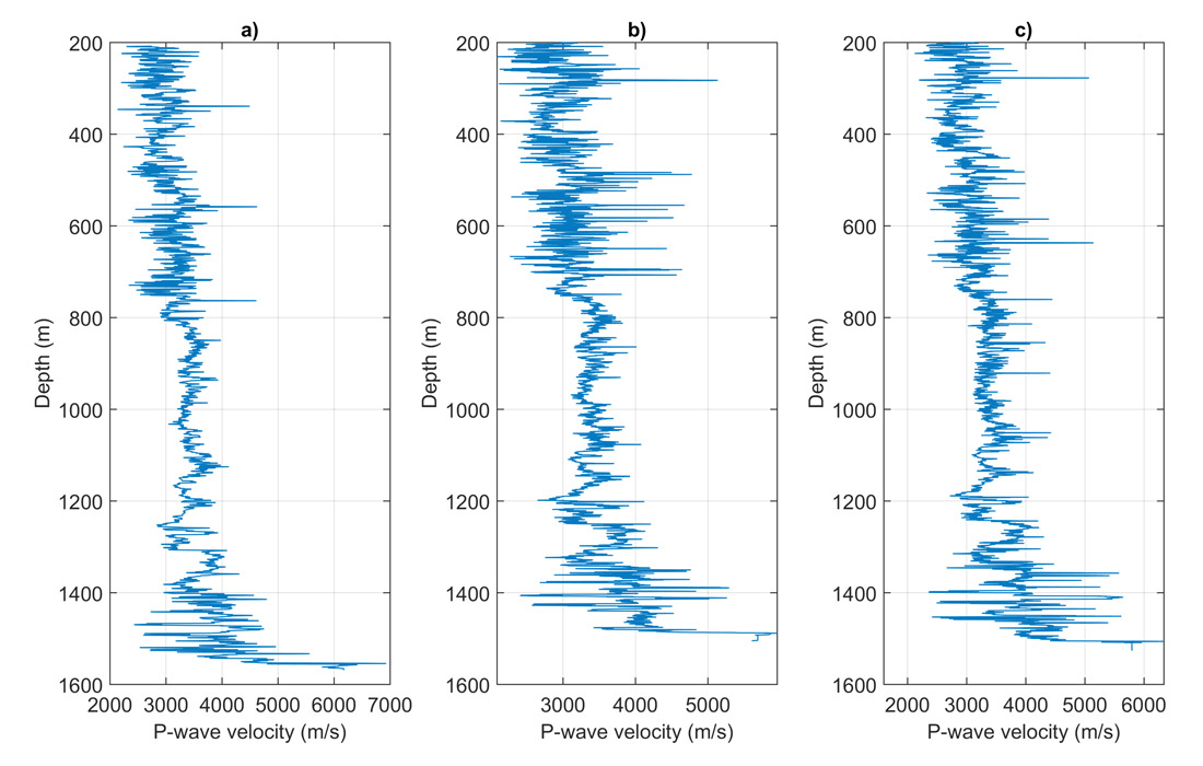
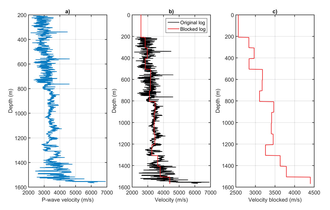
With the aim of maximizing the low frequency content of both sources and sensors, the Consortium for Research in Elastic Wave Exploration Seismology (CREWES) carried out an experimental seismic shoot at Hussar, Alberta in September, 2011. The seismic line was 4.5 km in length, running NE-SW and crossing (or nearly crossing) 5 wells named: 5-27, 12-27, 14-27, 1-34, and 14-35 (Margrave et al. 2012). See Figure 2. Three of the wells (12-27, 14-27, 14-35) were used to build two different Hussar synthetic models that were subsequently used to generate synthetic seismic data. The sonic logs of these wells are illustrated in Figure 3. These synthetics allow us to consider the plane-wave domain multiple prediction in situations with multiples generated by realistic geological models.

Synthetic 1: 100m blocked well 12-27

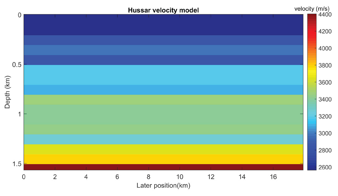
The P-wave sonic log of well 12-27 was blocked in 100 m intervals to build the first multi-layered velocity model, as shown in Figures 4 and 5. The velocity from surface to 200 m depth is a constant 2563 m/s.

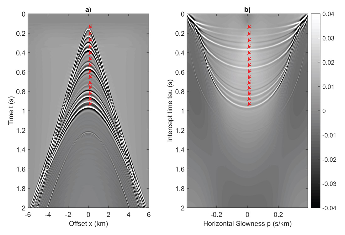
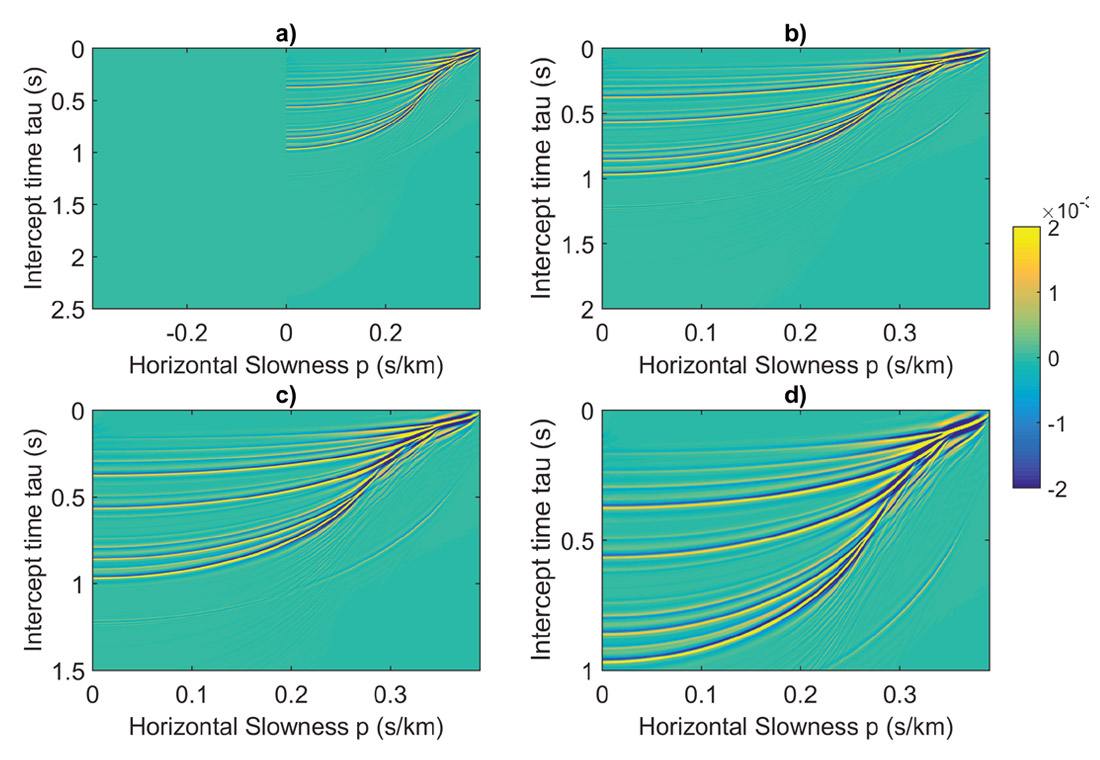
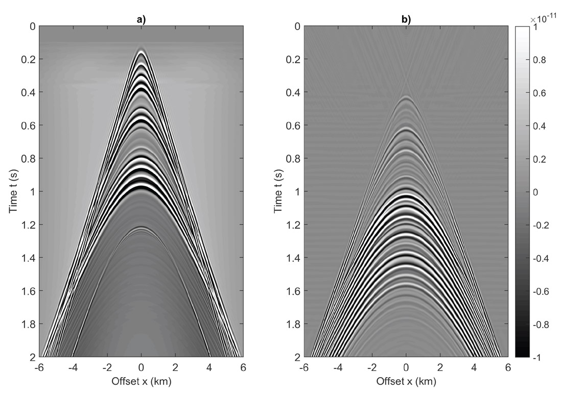
With four absorbing boundaries, finite difference synthetic data are created from the velocity model illustrated in Figure 5. A shot record with a source point at the centre is illustrated in Figure 6a. With the top of the model also absorbing, no free-surface multiples are created, only primaries and internal multiples. Primaries are indicated by red arrows. After a standard τ-p transform of this data set is calculated (Figure 6b), the transformed data set is adjusted by multiplying with –2iωq_s to produce the correctly scaled input for inverse scattering series internal multiple attenuation algorithm. The input to the prediction is illustrated in Figure 7. Each panel represents the transformed data truncated at a particular maximum travel time and slowness; minimizing can significantly reduce the computational burden. Notice that the events maintain a more or less constant width in the vertical time direction as the horizontal slowness grows, an indication that stationarity with respect to the optimum search parameter ε has been achieved (for further discussion of nonstationarity in ε, see Innanen, 2016).

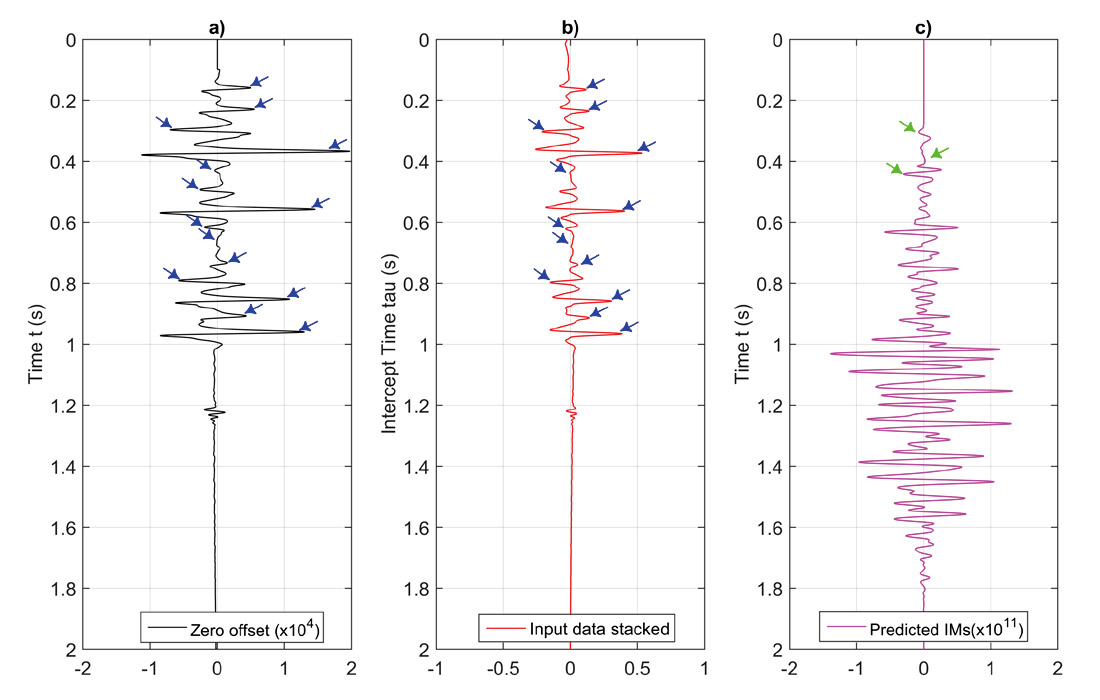
After the prediction algorithm, an inverse τ-p transform was applied to bring the predicted internal multiples to the time-offset domain, as shown in Figure 8. A detailed comparison between the raw zero-offset trace, the stacked input trace, and predicted zero-offset internal multiple trace is shown in Figure 9. Three important internal multiples are: the first-order multiple in the second layer, the second-order multiple in the second layer, and the first-order multiple in the third layer. These are indicated by green arrows in Figure 9c. The first three internal multiples interfere with the three primaries described above, as indicated by blue arrows in Figure 9a and 9b. These results indicate that the prediction algorithm estimated the correct travel time of all possible internal multiples, but with varying amplitudes, which means an adaptive subtraction will be needed to remove internal multiples from original data.

Hussar synthetic with 3 wells: 12-27, 14-27, and 14-35

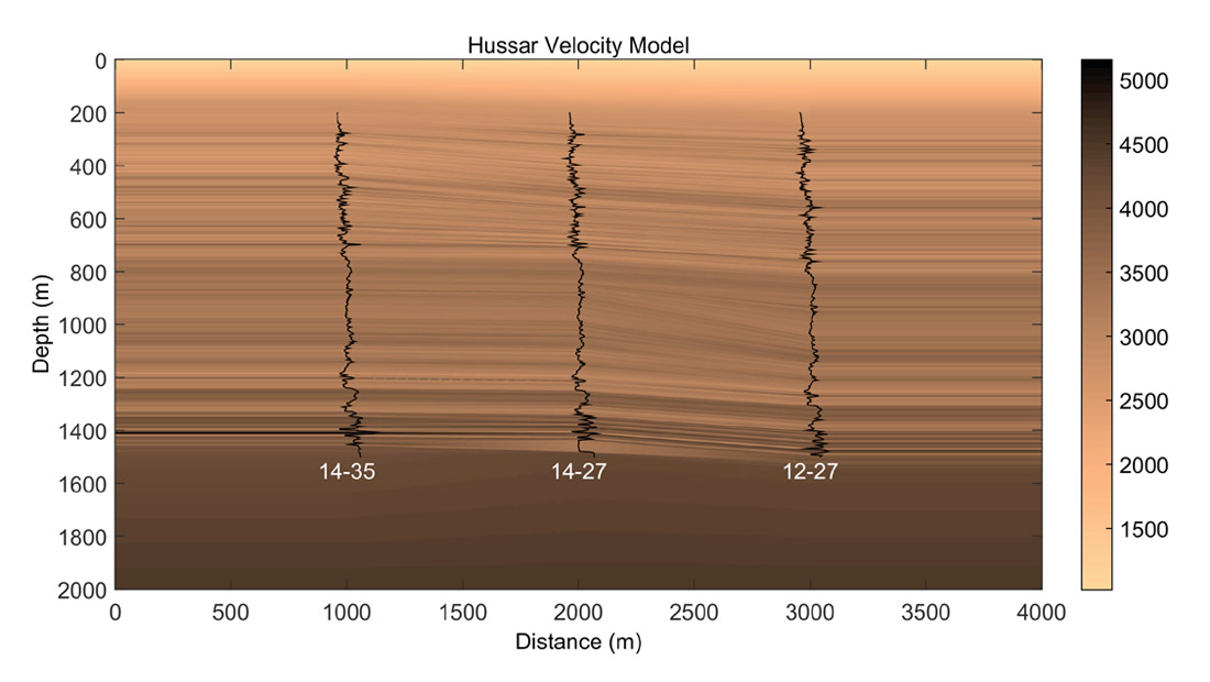
Interpolation was used to simulate a geological medium between well logs along the Hussar 2D seismic line, as published by Margrave (2015). The Hussar seismic line was shot through wells 12-27, 14-27, and 14-35 from southwest to northeast. The three well logs all start at approximately 200 m in depth, and extend to about 1550 m. The spatial locations of the 3 wells in Figure 10 are chosen for convenience, and to generate realistic 2D geology, but do not represent their actual positions along Hussar seismic line of Figure 2. An inverse distance weight was applied to create interpolated logs between 2 wells, and formation tops guided the change between horizons through stretching and squeezing. To produce realistic overburden (the upper 200 m) and underburden (from log bottom to 2000 m depth) structures, a linear gradient was used from the uppermost available value at log top to 1000 m/s for the overburden, and from the lowermost available value at log bottom to 4500 m/s for the underburden (Margrave, 2015). The interpolated Hussar velocity model is shown in Figure 10.

Acoustic finite difference code was used to create a set of 61 shot records with source interval of 66.7 m, and receiver interval of 2.5 m. A minimum phase wavelet with a dominant frequency of 50 Hz was applied to create synthetic shot records. Before CMP stacking, a f-k fan filter was applied to remove ground roll and surface-related noise. Figure 11 shows the CMP stack of the synthetic section. Note that every event below 1.1 s is an internal multiple. All internal multiples can be predicted by implementing equation 1 in a shot by shot manner, as shown in the previous example. However, the prediction algorithm can also be applied on post-stack seismic data by reducing the dimensionality of equation 1, i.e., p_g = p_s=0 for 1D case. The CMP stacked section in Figure 11 was treated as 1D case, trace by trace in the processing of prediction.

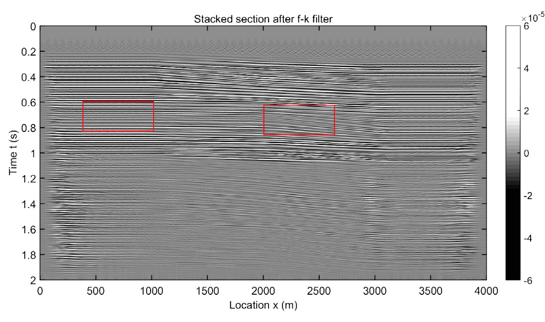
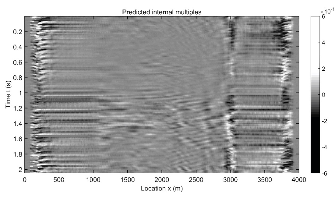
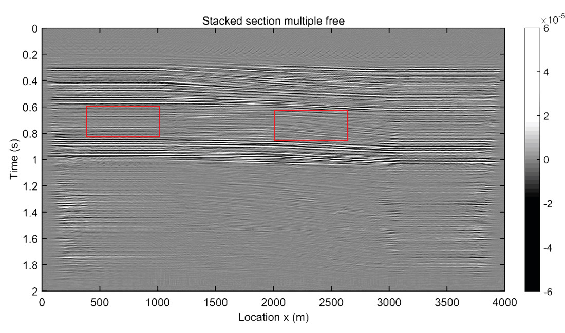
Predicted internal multiples on the CMP stacked section are illustrated in Figure 12. Adaptive subtraction was then applied to remove the internal multiples from the CMP stacked section. The result is shown in Figure 13. Compared to the raw CMP stacked section, the multiple-free CMP stack has significant advantages below 1.1 s, and internal multiple interference with primary events is also attenuated above 1.1 s (see rectangles in Figures 11 and 13). The multiple prediction is very “clean” and without domain related artifacts, making it a suitable input to a very mild adaptive subtraction process which has minimal effects on primaries.

Conclusion

The inverse scattering series internal multiple attenuation algorithm can predict internal multiples caused by unknown (or imperfectly known) generators in an unknown media. Predictions absent of almost all transform/aperture related artifacts are achieved by implementing the prediction in the plane wave domain. This domain also leads to a requirement for a relatively stationary search parameter, which makes for less interpretive intervention and thus an algorithm that proceeds more automatically. We exemplify the algorithm with synthetic land datasets in plane wave domain, noting an absence of artifacts. The plane-wave domain inverse scattering series predictions appear to be well-suited to the problem of cleanly separating primary and multiple events in a waveform consistent manner. The latter feature will be critical to future uses of predictions as means to selectively regulate and analyze residuals in full waveform inversion.

Acknowledgements

The authors thank Scott Keating for discussions and help on the adaptive subtraction method. This work was funded by CREWES industrial sponsors and NSERC (Natural Science and Engineering Research Council of Canada) through the grant CRDPJ 461179-13.